We investigate optimal strategies for reallocating investments from a risk-free asset class $B$ to a risky asset class $S$ that offers higher average returns but also comes with greater volatility. The primary objective is to determine the optimal trade-off between maximizing returns and minimizing volatility over a one-year period. We explore whether it is more advantageous to move all assets from $B$ to $S$ at the beginning of the year or to distribute the reallocation in portions over time. The results can be reproduced with the code in this GitHub Gist and Colab Notebook.

1. Problem description
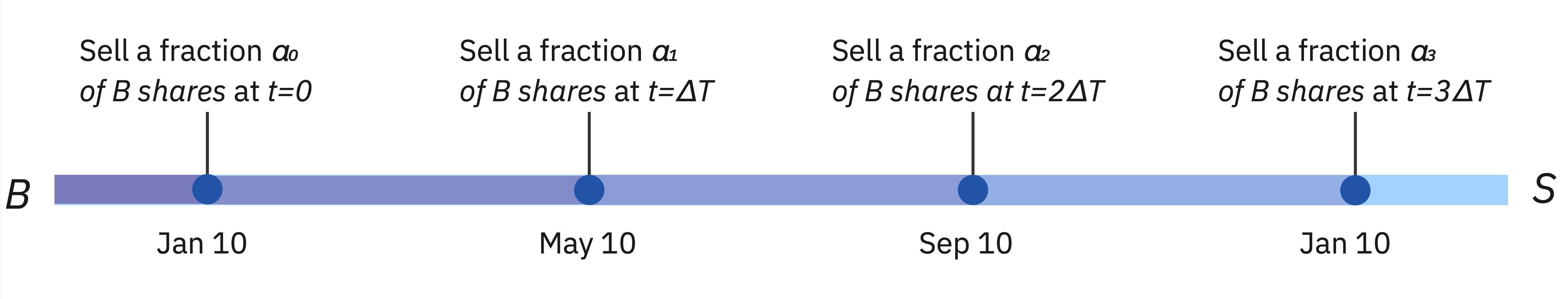
Assume that initially all investments are allocated in an asset class $B$ which has a fixed return rate $r$. A second asset class $S$ has higher average return rate $\mu$ than $B$ but comes with higher volatility: there is a chance that its returns are much lower than $r$. The goal is to transition all assets to $S$ within one year. This is done at equidistant points in time $\{t_j |j=0, \ldots N\}$ by transferring fractions $\{ \alpha_j | j=0, \ldots N\} $ of the initial investment in $B$ to $S$. For example, if we decide to do this operation once every 4 months then the fractions are described by a 4-dimensional vector $\alpha=[\alpha_0, \alpha_1, \alpha_2, \alpha_3]$ whose elements are non-negative and sum up to $1$: we sell $B$ and buy $S$ at the 0th, 4th, 8th and 12th month of the time interval. A graphical description for the case where the time span between two sell events $\Delta T$ is 4 months is provided below.
We are interested in the overall portfolio's growth $G$ in the end of the one-year interval. It is given by:
\begin{align} \label{eq:g_definition} G & = \sum^{N}_{n=0} \alpha_n \frac{ B(n \, \Delta T) }{ B(0) } \frac{ S(N \, \Delta T) }{ S(n \, \Delta T ) } \end{align}Each term in \eqref{eq:g_definition} describes the relative value growth of investments initially allocated in $B$ and then moved to $S$ at $n\Delta T$. The first fraction is the relative growth of $B$ from $t=0$ to $t=n\Delta T$ (the time we sell this asset) and the second fraction - the relative growth of $S$ from $n\Delta T$ to $N\Delta T$ (the end of the one-year window). In the previous example $\Delta T=4$ months and $N=3$.
Since the time evolution of $S$ is described by a stochastic process, the fractions $S(N\Delta T)/S(n \Delta T)$ are random variables, and hence the portfolio's growth $G$ is a random variable, as well. We want to understand how the mean, standard deviation (std) and particular percentiles of the probability distribution describing $G$ change as we change the allocation strategy $\alpha$. Intuitively, we know that achieving higher average returns is at the cost of higher std, and worse worst case performance scenarios (described by the low percentiles of the $G$-distribution). Nevertheless, there are strategies that offer the same average returns as other strategies but with a lower volatility, and we would like to identify them.
2. Time evolution of the asset classes
As mentioned in the previous section, the two asset classes $B$ and $S$ have different behaviour. The risk-free asset $B$ provides a constant return rate $r$, leading to predictable exponential growth. Conversely, the risky asset $S$ is modeled using a Geometric Brownian motion, characterized by a drift parameter $\mu$ and a volatility parameter $\sigma$. The time evolution of $B$ is straightforward, represented by the equation
\begin{align} B_t &= B_0 \, \exp(r \, t) \end{align}For the risky asset $S$, we describe its random fluctuations over time with the stochastic differential equation
\begin{align} dS_t & = \mu \, S_t \, dt + \sigma \, S_t \, dW_t \end{align}where $W_t$ is a Wiener process. The solution to this equation is given by:
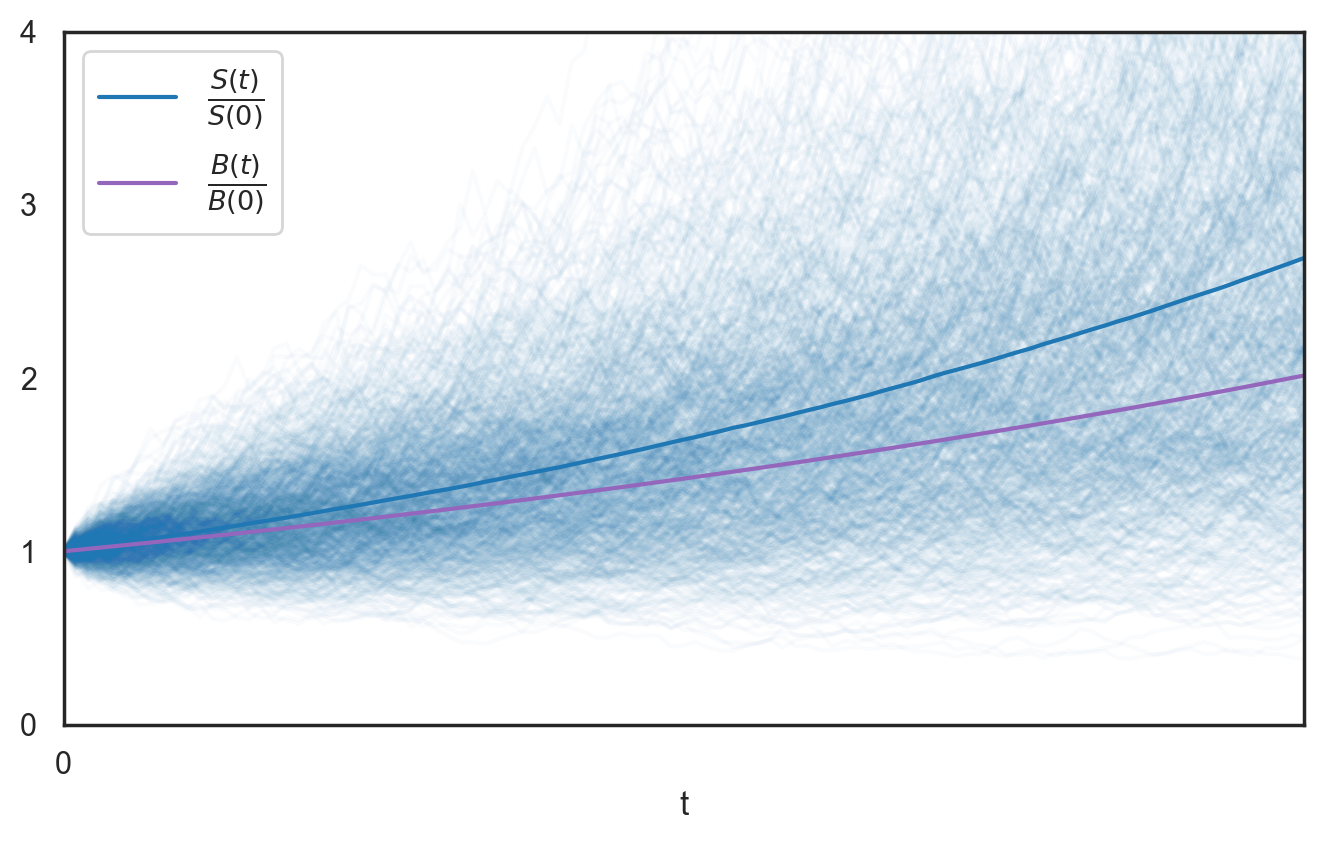
\begin{align} \label{eq:s_solution} S_t &= S_0 \, \exp( (\mu - \sigma^2/2) \, t + \sigma \, W_t) \end{align}Drawing the time evolution of $B_t$ is straightforward. On the other hand, to visualize the evolution of $S_t$ we simulate multiple trajectories of its stochastic process, allowing us to observe the variability in outcomes, as shown in the figure below.
3. Solution of the optimization problem
To understand how the distribution of $G$ given $\alpha$ looks like, we have to sample many trajectories of the process $S_t$, and calculate $G$ for each one of them. Then we can examine the resulting histogram of results to calculate the metrics we are interested in such as mean, std, and percentiles. In the appendix we demonstrate how to sample trajectories of $S_t$ and use them to generate samples of $G$.
In the following experiments we measure the time in units of years ($N\Delta T=1$ and $\Delta T=1/N$) and set $(r, \mu, \sigma) = (0.03, 0.09, 0.14)$ which means that the relative growths $B_t/B_0$ and $S_t/S_0$ satisfy the following relations after one year:
\begin{align*} \frac{B(1)}{B(0)} & = \exp(r) \approx 1.03 \\ \mathbb{E} \left[ \frac{S(1)}{S(0)} \right] & = \exp(\mu) \approx 1.09 \\ \text{STD} \left[ \frac{S(1)}{S(0)} \right] & = \exp(\mu) (\exp(\sigma^2) - 1)^{1/2} \approx 0.15 \end{align*}i.e. an investment in $B$ or $S$ is expected to yield an average annual growth of $3\%$ or $9\%$, respectively. These figures are typical for returns from a bank savings account or an index fund investment.
Given this insight, what typical values can we expect for $G$? The mean and standard deviation of $G$ should always fall between the corresponding metrics of $B_t/B_0$ and $S_t/S_0$ as shown below:
\begin{align} \label{eq:g_inequalities} \frac{B(1)}{B(0)} & \le \mathbb{E} \left[ G \right] \le \mathbb{E} \left[ \frac{S(1)}{S(0)} \right] & 0 & \le \text{STD} \left[ G \right] \le \text{STD} \left[ \frac{S(1)}{S(0)} \right] \end{align}Obtaining the lowest possible mean and standard deviation is achieved by delaying the reallocation of all $B$ assets until the very end of the year, represented by $\alpha = [0 \ldots 0, 1]$. Conversely, to reach the highest limits, we reallocate all $B$ assets at the start of the year, represented by $\alpha = [1, 0 \ldots 0 ]$. This can be directly seen if we use the two $\alpha$-vectors in \eqref{eq:g_definition}:
\begin{align*} G & = \sum^{N}_{n=0} \alpha_n \frac{ B(n/N) }{ B(0) } \frac{ S(1) }{ S(n/N ) } = \begin{cases} \frac{ B(1) }{ B(0) }, & \text{if } \alpha=[0, \ldots 0, 1] \\ & \\ \frac{ S(1) }{ S(0) }, & \text{if } \alpha=[1, 0 \ldots 0] \\ \end{cases} \end{align*}3.1 Example: 4-step uniform reallocation
We examine the strategy of selling $25\%$ of our $B$ shares every 4 months (at the 0th, 4th, 8th, and 12th months), represented by $\alpha = [1/4, 1/4, 1/4, 1/4]$. The figure below shows the distribution of the relative growth $G$ after one year.
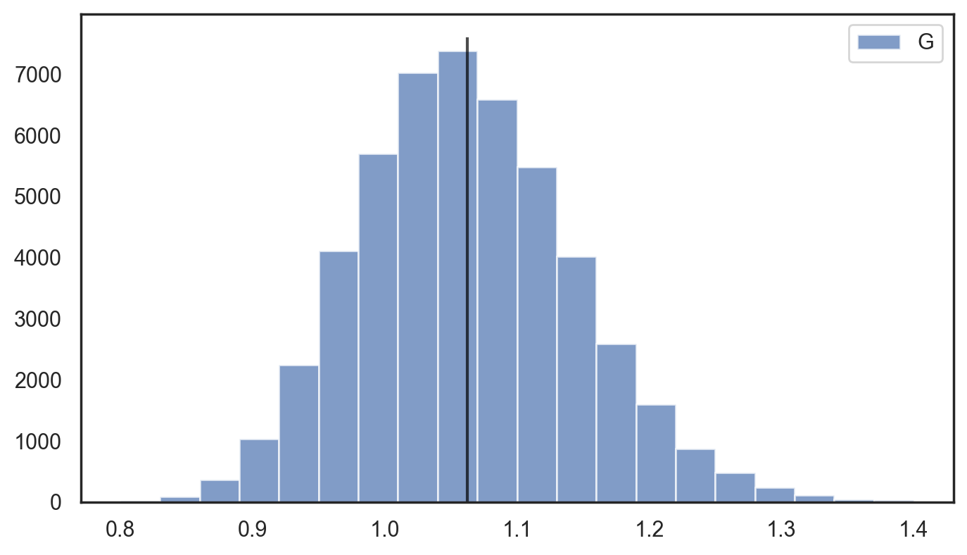
As expected, the mean relative return $\mathbb{E}[G]=1.062$ and the standard deviation $STD[G]=0.082$ fall within the expected ranges defined in \eqref{eq:g_inequalities}, with a $5\%$ and $10\%$ chance of the growth being below $93.6\%$ and $96.1\%$, respectively.
3.2 Arbitrary 4-step reallocation strategies
The example $\alpha = [1/4, 1/4, 1/4, 1/4]$ is just one of countless reallocation strategies. We use a Dirichlet distribution to randomly generate other $\alpha$ strategies and calculate the mean, standard deviation, and percentiles of the corresponding relative growth $G$. Results from $10,000$ strategies are plotted below.
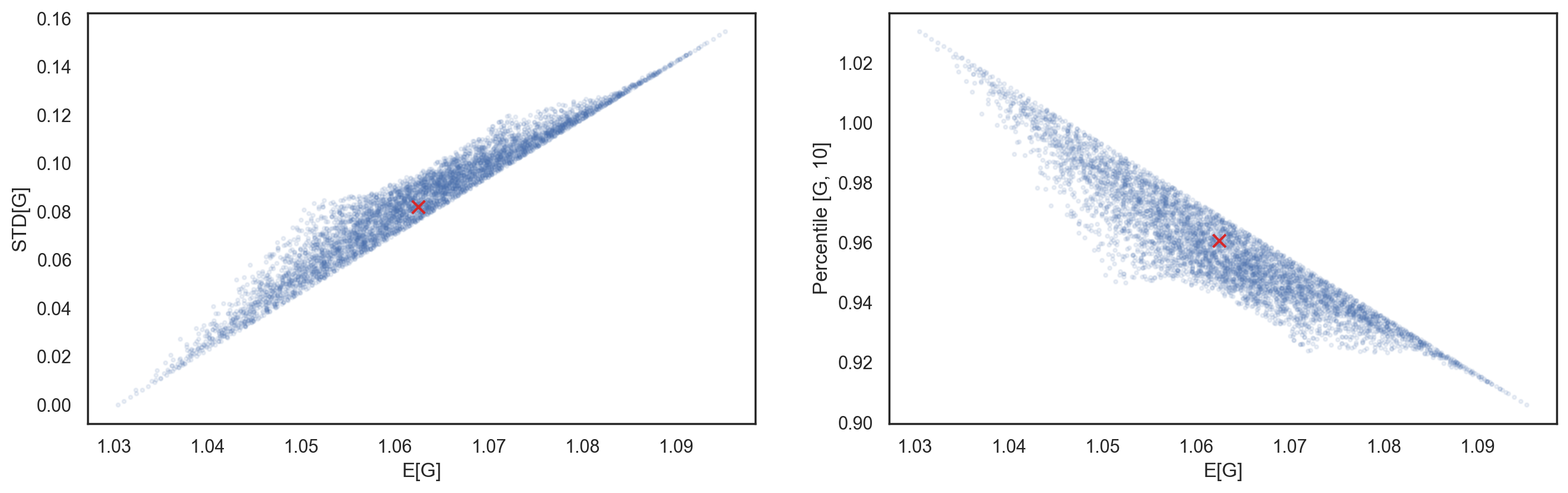
If we look at a vertical stripe of the left figure there will be many strategies with the same mean relative growth $G$ but with different std. For instance, at $\mathbb{E}[G] \approx 1.06$, some strategies have significantly lower standard deviations than the uniform strategy (marked by a red cross). We are interested in the subset that has the lowest $STD[G]$ given $\mathbb{E}[G]$. Based on the numerical results, all these optimal strategies follow the pattern:
\begin{align*} \alpha & = [c, \,\,\, 0, \,\,\, 0, \,\,\, 1-c] \hspace{7.0mm} 0 \le c \le 1 \end{align*}indicating reallocations occur only at the beginning and end of the year, with no action in the 4th and 8th months.
Similarly, when examining the 10th percentile of $G$ instead of $STD[G]$, the same pattern emerges for the optimal strategies.
3.3 Arbitrary m-step reallocation strategies
We can extend the experiment to arbitrary $m$-step reallocation strategies. For instance, we analyzed 7-step and 13-step strategies, corresponding to selling $B$ and buying $S$ every two months and every month, respectively. In both scenarios, the optimal strategy takes the form:
\begin{align*} \alpha & = [c, \,\,\, 0 \,\,\, \ldots \,\,\, 0, \,\,\, 1-c] \hspace{7.0mm} 0 \le c \le 1 \end{align*}We expect to see the same results for any other $m$-step strategy.
4. Summary
This article explores optimal strategies for reallocating assets from a risk-free asset class to a risky one with higher returns. It uses stochastic modeling, specifically Geometric Brownian motion, to analyze the time evolution of assets and compare different reallocation approaches. By simulating various strategies, it identifies the optimal allocation that balances return and volatility. The study finds that reallocating assets only at the beginning and end of the investment period minimizes risk while maximizing return potential.
Appendix
Drawing samples from G
We can reformulate the equation for relative growth $G$ from the first section as follows:
\begin{align*} G & = \sum^{N}_{n=0} \alpha_n \frac{ B(n \, \Delta T) }{ B(0) } \frac{ S(N \, \Delta T) }{ S(n \, \Delta T ) } \\ & = \sum^{N}_{n=0} \alpha_n \exp( r \, n \, \Delta T ) \exp \left( \log \left( \frac{S(N \, \Delta T) }{ S(0) } \frac{S(0) }{ S(n \, \Delta T) } \right) \right) \\ & = \sum^{N}_{n=0} \alpha_n \exp( r \, n \, \Delta T ) \exp \left( \log \left( \frac{ S(N \, \Delta T) }{ S(0) } \right) - \log \left( \frac{ S(n \, \Delta T) }{ S(0) } \right) \right) \end{align*}Instead of drawing samples from the process $S_t$ we use the transformed process $X_t = log(S_t/S_0)$, known as Arithmetic Brownian Motion:
\begin{align*} X_t & = (\mu - \sigma^2 / 2) \, t + \sigma \, W_t \hspace{8.0mm} X_0 = 0 \\ dX_t & = (\mu - \sigma^2 / 2) \, dt + \sigma \, dW_t \end{align*}To sample a trajectory of $X_t$ we use the Euler-Maruyama method with a small step size $\delta t$:
\begin{align*} X(t + \delta t) & = X(t) + (\mu - \sigma^2/2) \, \delta t + \sigma \, \sqrt{\delta t} \,\, \xi_t \hspace{8.0mm} \xi_t \sim \mathcal{N}(0, 1) \end{align*}where $\xi_t$ are independent normally distributed random variables sampled at every step. Typically, we have to use a very small step $\delta t$ to move forward in time. Since the drift $(\mu-\sigma/2)$ and diffusion $(\sigma)$ terms of the SDE are constants we can work with arbitrarily large $\delta t $. To demonstrate, consider moving from $t_0$ to $t_1$ in $N'$ steps. The step $\delta t =(t_1-t_0)/N'$ can become arbitrarily small for large $N'$:
\begin{align*} X(t_0 + \delta t) & = X(t_0) + (\mu - \sigma^2/2) \, \delta t + \sigma \, \sqrt{\delta t} \,\, \xi_1 \\ X(t_0 + 2\delta t) & = X(t_0 + \delta t) + (\mu - \sigma^2/2) \, \delta t + \sigma \, \sqrt{\delta t} \,\, \xi_2 \\ & = X(t_0) + (\mu - \sigma^2/2) \, 2 \, \delta t + \sigma \, \sqrt{\delta t} \,\, (\xi_1 + \xi_2) \\ & \vdots \\ X(t_0 + N'\delta t) & = X(t_0) + (\mu - \sigma^2/2) \, N' \, \delta t + \sigma \, \sqrt{\delta t} \,\, (\xi_1 + \ldots + \xi_{N'}) \end{align*}The sum in the last line $\xi_0 + \xi_1 + \ldots $ forms a normally distributed random variable with zero mean and variance $N'$, which can be reparametrized as $\sqrt{N'}· \varepsilon$, where $\varepsilon \sim \mathcal{N}(0, 1)$. If we use this expression in the last line of the previous equation we get:
\begin{align*} X(t_1) & = X(t_0) + (\mu - \sigma^2/2) \, (t_1 - t_0) + \sigma \, \sqrt{t_1 - t_0} \,\, \varepsilon \hspace{8.0mm} \varepsilon \sim \mathcal{N}(0, 1) \end{align*}This formula allows us to sample $X_t$ at the time ordered points $(t_0, t_1, t_2 \ldots) = (0, \Delta T, 2 \Delta T \ldots)$. From each sampled $X$-trajectory we can compute $G$:
\begin{align*} G & = \sum^{N}_{n=0} \alpha_n \exp \big( r \, n \, \Delta T \big) \exp \big( X(N\Delta T) - X(n\Delta T) \big) \end{align*}The code to generate samples of the Arithmetic Brownian Motion is provided below: