Table of Contents
Employing a Variational Inference approach, we perform regression on a continuous variable $Y$ and its associated uncertainty, denoted by $STD[Y]$, utilizing a set of categorical features. Given the potential magnitude of the dataset, consisting of millions of events, we simplify the likelihood function of the model to enhance numerical stability and accelerate solutions. The implementation of this solution with Tensorflow Probability is available in the dedicated Github repository and Colab notebook.
1. Problem definition
Let’s examine the task of utilizing $M$ categorical features to forecast both the mean value and standard deviation of a target variable $Y$. A straightforward approach involves employing a linear function (augmented by an exponential or softplus link function for the non-negative standard deviation) to model both target variables. Upon applying one-hot encoding to each feature and transforming them into vectors with dimensions equal to the cardinality of the respective features, we can characterize them as follows:
\begin{align} \label{eq:regr_1a} f(x, b) & = \sum^{M-1}_{u=0} \vec{b}_u \cdot \vec{x}_u, \\ \label{eq:regr_1b} g(x, a) & = \text{softplus} \left( \sum^{M-1}_{u=0} \vec{a}_u \cdot \vec{x}_u \right) \end{align}where $f$ models the mean, $g$ — the standard deviation, $x_u$ — the one-hot encoded feature $u$, and $a_u$, $b_u$ — the yet to be learned weights.
The priors of the individual elements $b_{uv}$ in \eqref{eq:regr_1a} (1a) are characterized by normal distributions $\rho (b_{uv} | 0, \lambda^2_{uv})$ with a mean of zero and a standard deviation of $\lambda_{uv}$. To ensure positivity, $\lambda_{uv}$ is drawn from a Gamma distribution, $\Gamma(\lambda_{uv}| \alpha, \beta)$, where $\alpha$ is the shape parameter and $\beta$ is the rate, both constants. The priors for the weights $\alpha_{uv}$ in \eqref{eq:regr_1b} are established in an identical manner. For a comprehensive overview of the introduced variables and their interdependencies, refer to the figure below.
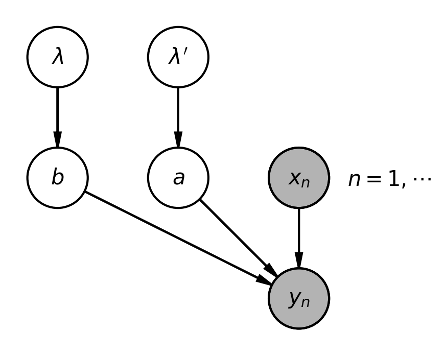
Let’s delve into the precise mathematical definitions of each term. The section on the left side of the graph, featuring the $\lambda$ and $b$ symbols, represents the prior distribution for the weights $b_{uv}$:
\begin{align} P(b | \lambda )P(\lambda) & = \prod^{M-1}_{u=0} \prod_{v} P(b_{uv} | \lambda_{uv})P(\lambda_{uv}) \nonumber \\ & = \prod^{M-1}_{u=0} \prod_{v} \rho \left(b_{uv} | 0, \lambda^2_{uv} \right) \gamma( \lambda_{uv} | \alpha_0, \beta_0), \hspace{5mm} \alpha_0= \beta_0 = 0.001 \end{align}The central portion refers to the priors of the $a_{uv}$ weights, and as previously noted, they are described in an identical manner as the $b_{uv}$ weights: a simple substitution of $b$ with $a$ and $\lambda$ with $\lambda'$ suffices.
Concluding the graph is the segment dedicated to the likelihood function, $P(y| x, a, b)$, modeled as the product of normal distributions $\rho(y| \mu, \sigma^2)$ for each data point $(x, y)$. Here, $\mu$ is determined by the function $f(x,b)$ in \eqref{eq:regr_1a}, and $\sigma$ is determined by $g(x,a)$ in \eqref{eq:regr_1b}.
2. Simplification of the likelihood function
With Tensorflow Probability, defining the joint-probability distribution function and its log-probability is straightforward, and the application of the variational inference approach is exemplified in the subsequent section.
Unfortunately, this implementation experiences escalating convergence times as the dataset size grows. To mitigate computational demands, a time-saving strategy involves simplifying the log-likelihood expression. Subsequently, we can substitute the original likelihood distribution in the solution with a newly devised custom distribution object housing the adjusted log-likelihood expression.
When dealing with only $M$ categorical features, the data points in the training dataset can be organized into a finite number of groups. Each group corresponds to a unique combination of values that the categorical features can take. The total number of groups, $N$, is equal to or less than the product of the cardinalities of the features. For example, if we have a categorical feature that can take $2$ unique values and another one that can take $4$ unique values, the total number of groups should be $8$. Here, the index $i$ denotes the group, and $j$ represents an index within that group. All observations can be expressed as $\{ (y^{(ij)}, x^{(ij)}) | i = 1, \ldots N, j = 1, \ldots N_i \}$, where $N_i$ denotes the number of elements in group $i$, and $x^{(ij)}$ refers to all categorical features of observation $(ij)$. Since all elements within the same group $i$ share identical categorical features, we can simplify $x^{(ij)}$ to $x^{(i)}$.
The likelihood function in \eqref{eq:likelihood} could be rewritten in the following form:
\begin{align*} P(y|x, a, b) & = \prod^{N}_{i=1} \prod^{N_i}_{j=1} \rho \left( y^{(ij)} \Big| f(x^{(ij)}, b), g^2(x^{(ij)}, a) \right) \\ & \propto \exp \left[ -\frac{1}{2} \sum^{N}_{i=1} \sum^{N_i}_{j=1} \frac{ \left( y^{(ij)} - f(x^{(ij)}, b) \right)^2 }{ g^2(x^{(ij)}, a) } \right] \\ & \propto \exp \left[ -\frac{1}{2} \sum^{N}_{i=1} \frac{N_i}{ g^2(x^{(i)}, a) } \bigg( f^2(x^{(i)}, b) - 2 \cdot f(x^{(i)}, b) \cdot \mathbb{E}\left[y^{(i)}\right] + \mathbb{E}\left[y^{(i)2}\right] \bigg) \right] \\ & \propto \exp \left[ -\frac{1}{2} \sum^{N}_{i=1} \frac{N_i}{ g^2(x^{(i)}, a) } \bigg( \big( f(x^{(i)}, b) - \mathbb{E}\left[y^{(i)}\right] \big)^2 + \underbrace{ \mathbb{E}\left[y^{(i)2}\right] - \mathbb{E}\left[y^{(i)}\right]^2 }_{ STD \left(y^{(i)} \right)^2 } \bigg) \right] \\ \mathbb{E}\left[y^{(i)}\right] & \equiv \frac{1}{N_i} \sum^{N_i}_{j=1} y^{(ij)} \\ \mathbb{E}\left[y^{(i)2}\right] & \equiv \frac{1}{N_i} \sum^{N_i}_{j=1} y^{(ij)2} \end{align*}The last line of the equation was derived by adding and subtracting $\mathbb{E} [y^{(i)}]^2$ and regrouping the terms.
The derivation of the log-probability for both the likelihood component and the complete joint-probability distribution function \eqref{eq:likelihood} is straightforward. All summations involved are solely over the $N$ distinct groups. Within each group, the observed target values $y^{(ij)}$ are replaced with the group mean, $\mathbb{E}[y^{(i)}]$, and standard deviation, $STD[y^{(i)}]$. The resulting number of elements $N$ is considerably smaller than the total count of original observations $\sum_i N_i$.
3. Example
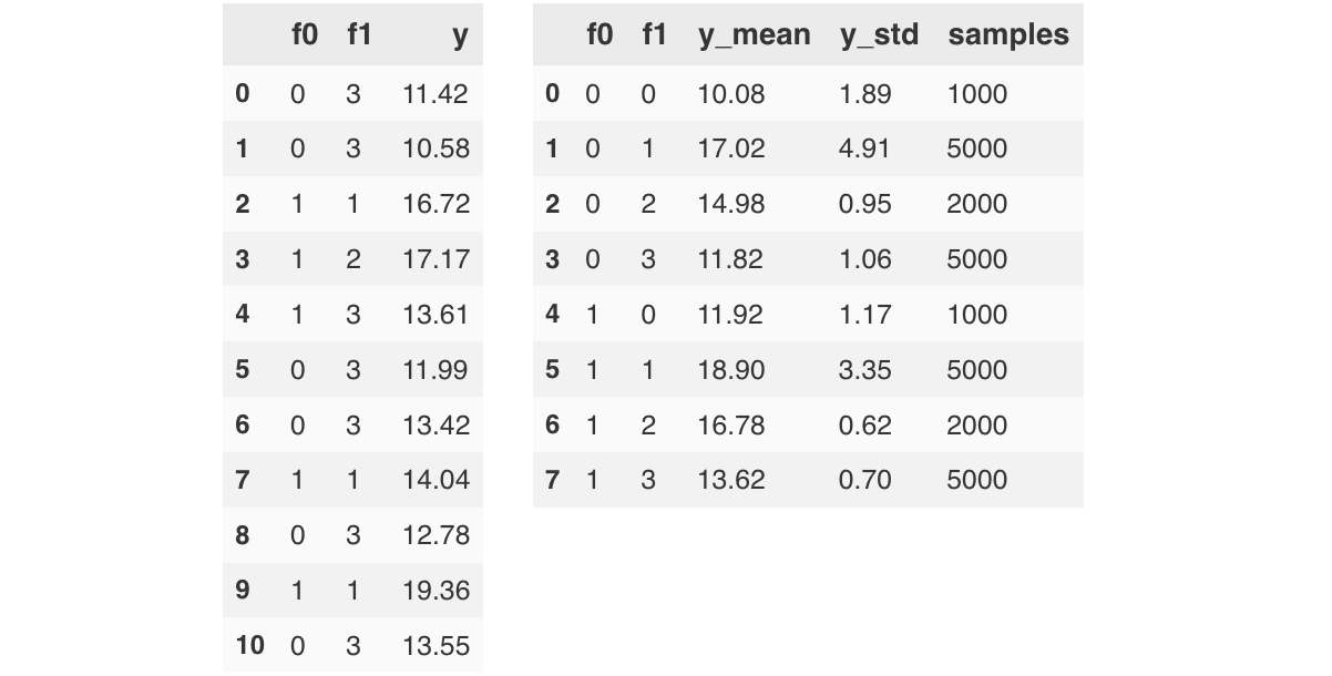
We explore a scenario of having a target variable $Y$ whose mean and standard deviation can be linearly regressed by two categorical variables $f0$, $f1$ with cardinalities of $2$ and $4$, respectively (and with a softplus link function applied to the standard deviation). The figure below provides a sample of the generated data:
3.1 Standard solution
To build the model (the joint probability distribution in \eqref{eq:likelihood}) we can use the code snippet below:
Since we are using the Variational inference approach to solve the problem, we have to construct a surrogate posterior for $\lambda_{uv}$, $\lambda'_{uv}$, $a_{uv}$, $b_{uv}$, as well. For simplicity, we assume that that there are no correlations between the variables. This reduces the posterior description to the product of univariate distributions of the normally distributed weights $a_{uv}$, $b_{uv}$ and log-normally distributed $\lambda_{uv}$, $\lambda'_{uv}$.
The code snippet below demonstrates how the model is trained with (method=aggregated)
and without (method=standard) the likelihood simplification. Between the two approaches
there are almost no differences, except the use of build_model_agg_data()
and build_model() to construct the likelihoods, and the different input data.
3.2 Solution with modified likelihood
We can use the same definition of the priors and the surrogate posteriors from
the previous solution. The only difficulty is plugging in the new likelihood
function into the joint distribution. To achieve this we create a new class
derived from the standard AutoCompositeTensorDistribtuion Tensorflow class.
We are interested only in the log_prob() method of this class. The method to
sample values from the distribution is defined only because Tensorflow uses it
to infer the right dimensions of the sampled values (so it is fine if we define
it to return only zeros).
The model (joint probability distribution) is build similarly to the model from the standard solution:
3.3 Scaling of both approaches
One can use this Colab-notebook to check if the predicted mean and standard deviation of the target variable for all feature combinations between both models are the same. By increasing the dataset size one can see that the computation time of the solution employing the modified likelihood is constant. On the other hand the computation time of the standard solution significantly increases.
4. References