We explain the application of the Bayesian inference approach, described in the previous blog post, to the case of having multiple trajectories of a stochastic process. We will consider an analytically solvable problem to address the question of how much the past values of a trajectory reduce our uncertainty about its future values. In addition, we will also solve the problem using the MCMC approach, implemented in the Tensorflow probability library, and compare both results.
1. Stochastic processes and State space models
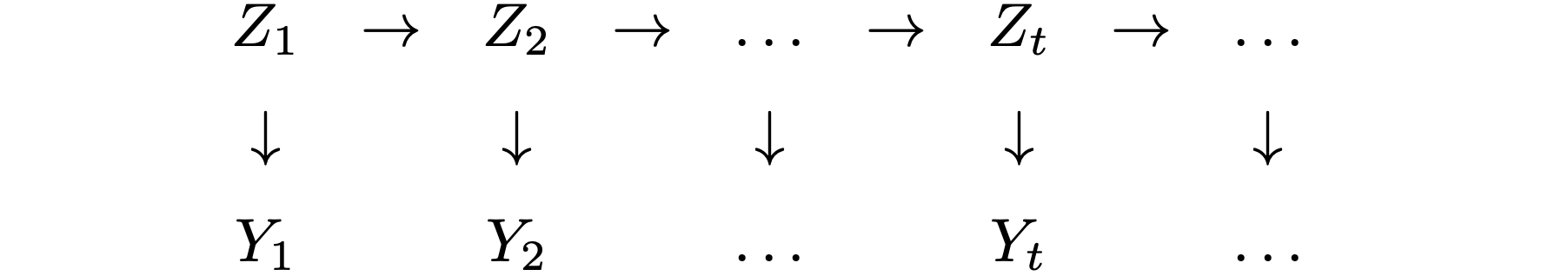
A stochastic process can be defined as a collection of random variables $\{Z_t\}$ with a time index $t$. To obtain some information from it we often make observations $\{ y_t \}$ at different times that are noisy and deviate from the exact values $\{ z_t \} $. This type of problems is often described through state-space models where the observations $\{ y_t \}$ are described as samples of an observation process $\{ Y_t \}$ that depend linearly on the state process $\{ Z_t \}$. A graphical representation of the idea is given in the figure below:
To make everything more understandable, we will consider the local level model with a constant drift:
\begin{align} Y_t & = Z_t + \varepsilon_t \nonumber \\ \label{eq:loc_level} Z_t & = Z_{t-1} + \omega + \eta_t, \hspace{4.0mm} Z_0 = 0 \nonumber \\[2.0mm] \varepsilon_t & \sim \mathcal{N} \left( 0, \sigma^2_y \right), \hspace{10.2mm} \mathbb{E}\left(\varepsilon_t \varepsilon_{t'} \right) = 0 \hspace{2.0mm} \text{for} \hspace{2.0mm} t \neq t' \nonumber \\ \eta_t & \sim \mathcal{N} \left( 0, \sigma^2_z \right), \hspace{10.2mm} \mathbb{E}\left(\eta_t \eta_{t'} \right) = 0 \hspace{2.0mm} \text{for} \hspace{2.0mm} t \neq t' \end{align}which is constructed with the help of the normally distributed random variables $\varepsilon_t$, $\eta_t$, and with the constant $\omega$. Due to the noise term $\varepsilon_t$ our observations can be slightly below/above the true value of $Z_t$. We can eliminate $Z_t$ dependency in $Y_t$:
\begin{align*} Y_t & = \omega t + \sum^{t}_{\tau=1} \eta_{\tau} + \varepsilon_t \end{align*}Since $Y_t$ is a linear combination of Gaussian random variables it is also Gaussian with the following properties:
\begin{align} \mathbb{E}(Y_t) & = \omega t , \nonumber \\ {\rm cov} (Y_t, Y_{t'}) & = \min(t, t')\sigma^2_z + \delta_{tt'} \sigma^2_y, \end{align}where $\delta_{mn}$ is the Kronecker delta which is equal to $1$ if $m=n$ and to $0$ otherwise. One can also show that $\{ Y_t \}$ is a Gaussian stochastic process which means that the joint probability distribution of every sampled trajectory $\mathbf{y}$ $(\mathbf{y} = y_1 \ldots y_T)$ can be described as a multivariate normal distribution $\rho_{\mathcal{N}}(\mathbf{y} | \mathbf{\mu}, \Sigma)$ with mean $\mathbf{\mu}$ and covariance matrix $\Sigma$:
\begin{align} p (\mathbf{y}) & = \rho_{\mathcal{N}} \left( \mathbf{y} | \mathbf{\mu}, \Sigma \right), & & \mathbf{y}, \mathbf{\mu} \in \mathbb{R}^T \hspace{3.0mm} \Sigma \in \mathbb{R}^{T\times T} \nonumber \\ \mathbf{\mu}_t & = \mathbb{E}(Y_t) & & \nonumber \\ \Sigma_{tt'} & = {\rm cov} (Y_t, Y_{t'}) & & t,t' = 1, \ldots T \end{align}Because $\Sigma$ is not a diagonal matrix we cannot factorize $p(\mathbf{y})$ into a product of the distributions for each point of the trajectory $\mathbf{y}$. In fact, we can show that knowing $y'$ measured at $t' < t$ influences our measurement $y$ at $t$. We just have to compare the normal distributions $p(y|y')$ and $p(y)$:
\begin{align} p(y |y') & = \rho_{ \mathcal{N} } \left(y | \tilde{\mu}_{tt'}, \tilde{\sigma}^2_{tt'} \right) \nonumber \\[2.5mm] p(y) & = \rho_{ \mathcal{N} } \left(y| \mu_t , \sigma^2_t \right) \nonumber \\[0.2mm] \tilde{\mu}_{tt'} & = \mu_t + \frac{t' \sigma^2_{z} }{ \sigma^2_{t'} } (y' -t'\omega ) \nonumber \\[0.2mm] \mu_t & = t \omega \nonumber \\ \tilde{\sigma}^2_{tt'} & = \sigma^2_t - \frac{(t' \sigma^2_{z})^2 }{ \sigma^2_{t'} } \nonumber \\[0.2mm] \sigma^2_t & = t \sigma^2_{z} + \sigma^2_y \end{align}If we compare $(4e)$ and $(4f)$ we see that the variance of $p(y|y')$ is smaller than the variance of $p(y)$, i.e. knowing $y'$ decreases our uncertainty about $y$. A comparison of both means in $(4c)$, $(4d)$ shows us that any deviation of $y'$ from its expected value $\omega t'$ shifts the expected value of $y$ in the same direction.
In real world applications we might have data from multiple trajectories of the same stochastic process. For the process that we have considered we can see that the joint probability distribution of the points from all trajectories factorizes into a product of joint probability distributions for every trajectory:
\begin{align} p( \mathbf{y}^1, \ldots \mathbf{y}^M ) & = \prod^{M}_{m=1} p( \mathbf{y}^m ) ,\nonumber \\ \mathbf{y}^m & = y^m_1 \hspace{1.5mm} \ldots \hspace{1.5mm} y^m_T, \end{align}where $\mathbf{y}^m$ refers to the values of the $m$-th trajectory. In other words, the trajectories do not interfere with each other.
2. Example
We consider again the problem of finding out the growth rate $\omega$ of the trees in the Black Forest national park by using a dataset that contains two measurements of the height of every tree (and its age) taken at different points in time that differ by several years. The trees growth will be described by the local level model with constant drift $\omega$ that was defined in $(1)$ (we will also close our eyes for the fact that the tree heights may become negative. In the end we are just imagining things and our imagination should not any have boundaries). Our prior belief about the non-negative three growth rate $\omega$ is described through an exponential distribution:
\begin{align} p(\omega) & = \lambda_0 \exp \left( - \lambda_0 \omega \right) \Theta(\omega), \hspace{4.0mm} \lambda_0 > 0 \end{align}where $\Theta (\omega)$ is the Heavyside step function that is equal to $1$ for $\omega > 0 $ and $0$ otherwise. The variances of $\varepsilon_t$ and $\eta_t$ will be considered as known and won’t be deduced from the data.
2.1 Analytical solution for a single tree
In this case we have only one trajectory with two points. We will denote by $y$, $y'$ the height of the tree taken at $t$, and $t'$ $(t > t')$, respectively. The corresponding trajectory $\mathbf{y}$ will be $\mathbf{y} = (y, y')$. The joint distribution of the trajectory $p(\mathbf{y})$ is given by the two-variate normal distribution $(3)$. It can be also interpreted as the likelihood function of getting the trajectory $\mathbf{y}$ given that the tree growth rate is $\omega$. We can use the Bayesian theorem to combine our prior belief about the growth rate in $(6)$ with the likelihood function $p(\mathbf{y})$:
\begin{align} p \left(\omega \big| \mathbf{y}\right) & = C \cdot p \left( \mathbf{y} \right) p\left( \omega \right) \nonumber \nonumber \\ & = C \cdot \rho_{\mathcal{N}} \left( \omega \,\Big| \, \frac{\mathcal{B}_{yy'yy'} - \lambda_0 }{ \mathcal{A}_{tt'} }, \mathcal{A}^{-1}_{tt'} \right) \Theta(\omega), \nonumber \\ B_{y y' t t'} & = \frac{ y t \sigma^2_{t'} + y' t' \sigma^2_{t} - t' \sigma^2_{z} (y t' + y' t) }{ \sigma^2_t\sigma^2_{t'} -t'^2\sigma^4_{z} } ,\nonumber \\ A_{tt'} & = \frac{ t^2\sigma^2_{t'} + t'^2\sigma^2_{t} - 2t'\sigma^2_{z} tt'}{ \sigma^2_t\sigma^2_{t'} -t'^2\sigma^4_{z}} , \nonumber \\ \sigma^2_t & = t \sigma^2_z + \sigma^2_y, \end{align}where $C$ is a normalization constant. As in the example from the previous blog post, the posterior is a Truncated Normal distribution. To get this result we just have to use the definition of the prior $p(\omega)$ and the likelihood $p(\mathbf{y})$, invert the 2x2 covariance matrix $\Sigma$ and regroup the terms. The longer the time-series is, the bigger is the $\Sigma$ matrix that has to be inverted.
2.2 Analytical solution for multiple trees
We will denote by $y^m$, $y'{}^m$ the height of the $m$-th tree $(m = 1 \ldots M)$ taken at $t_m$, and $t'_m$ $(t_m > t'_m)$, respectively. The corresponding trajectory $\mathbf{y}^m$ will be $\mathbf{y}^m = (y^m, y'{}^m)$. By making use of $(5)$, the likelihood function of all measurements is given by:
\begin{align} p \left( \mathbf{y}^1, \ldots \mathbf{y}^M \right) & = \prod\limits^{M}_{m=1} p \left( \mathbf{y}^m \right) = \prod\limits^{M}_{m=1} \rho_{\mathcal{N}} \left( \mathbf{y}^m | \mathbf{\mu}^m, \Sigma^m \right) \, p\left( \omega \right), \nonumber \\[0.5mm] \mathbf{\mu}^m & = \left[ \begin{array}{c} \omega t'_m,\\ \omega t_m \end{array} \right], \nonumber\\[0.5mm] \Sigma^m & = \left[ \begin{array}{cc} t'_m \sigma^2_z + \sigma^2_y & t'_m \sigma^2_z \\ t'_m \sigma^2_z & t_m \sigma^2_z + \sigma^2_y \end{array} \right] \end{align}The posterior distribution of $\omega$ obtained after taking into account the information of the height measurements of all trees is given by:
\begin{align} p \left(\omega \big| \mathbf{y}^1, \ldots \mathbf{y}^M \right) & = C \cdot p \left( \mathbf{y}^1, \ldots \mathbf{y}^M \right) p\left( \omega \right) \nonumber \\ & = C \cdot \rho_{\mathcal{N}} \left( \omega \,\Big| \, \frac{\mathcal{B} - \lambda_0 }{ \mathcal{A} }, \mathcal{A}^{-1} \right) \Theta(\omega), \nonumber \\ \mathcal{B} & = \sum^{M}_{m = 1} B_{y^m , y'^m , t_m, t'_m}, \nonumber \\ \mathcal{A} & = \sum^{M}_{m=1} A_{t_m, t'_m}, \end{align}where all terms in the sums in $(9b)$, $(9c)$ are defined in $(7b)$, $(7c)$.
2.3 Numerical solution
To solve the problem numerically we will use the MCMC implementation in TensorFlow Probability. The training data is obtained through generating multiple trajectories from $(1)$ and picking two random points from each one of them: the time difference between the different pairs of chosen trajectory points can be different. The exact details of the data generation, model definition and model training are provided in this GitHub Gist.
Here we will only briefly explain the part of the code responsible for the model definition.
The tfd.JointDistributionSequentialAutoBatched() concatenates the $\omega$ prior (first element
in the list) with the likelihood function, as described in $(9a)$. The likelihood function is a
product of $M$ two-variate normal distributions. To verify that the $M$ two-variate random variables
are independent, as expected in $(5)$, we can sample many values from them, calculate the covariance
matrix and confirm that it only contains $M$ 2x2 non-zero block-matrices on the diagonal. An
example can be found
here.
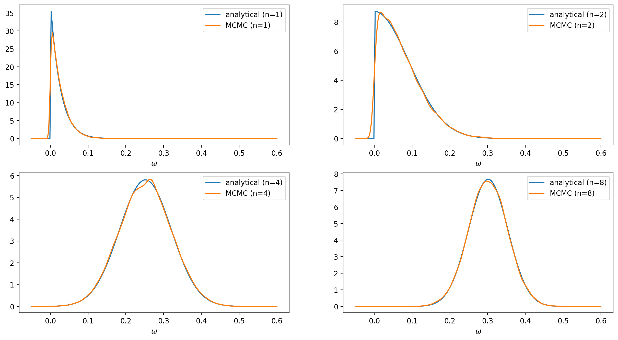
The analytical and numerical results for various numbers of trees are shown in the figure below. The impact of the prior on the $\omega$ posterior can be seen through the vertical cut at $\omega = 0$.
3 Final remarks
We have managed to solve a simple time series problem both analytically and numerically using the TensorFlow probability library. The code provided in the Gist can now be easily extended to longer time series.