The Bayesian inference approach gives us the opportunity to systematically combine and update our prior beliefs about the model parameters with new evidence. In the case where the prior and posterior are conjugate distributions, we can find either an exact analytic or a numerically inexpensive solution for the model parameters. In the more general cases, we must resort to the flexible but computationally intensive Markov chain Monte Carlo (MCMC) methods. Somewhere in between, we find the variational inference approaches, where we approximate the posterior with an easier-to-handle distribution that, depending on the choice, can still preserve some of the correlations between the model parameters. In this article we will take a deeper look at the variational inference approach, in particular, we will:
- explain the measure commonly used to quantify the difference between two distributions: the Kullback-Leibler divergence
- apply the variational inference and the MCMC approach to an analytically solvable problem
1. Variational inference approach
We are interested in the posterior distribution p of the parameters $\{ \omega_m \vert m =1, \ldots M \} $ of a model that is supposed to predict the outcome $y$ from the provided features $x$ \begin{align} \label{eq:init_eq} p \big( \omega | Y, X\big) & & \omega = [ \omega_1, \ldots \omega_M ]^T \end{align} by taking into account the new information from $N$ observations $(Y, X) \equiv \{( y^{(i)}, x^{(i)} ) \vert i = 1, \ldots N \}$ of the model performance. We want to approximate the posterior with a probability distribution function $q(\omega, \theta )$ where $\theta $ corresponds to a set of parameters whose value has to be determined.
A common choice for $q$ is the joint Gaussian probability distribution where all $\omega_m$ variables are independent of each other: \begin{align} q( \omega, \theta ) & = \prod\limits^{M}_{m=1} q( \omega_m, \theta_m ), \\ q( \omega_m, \theta_m ) & = \frac{1}{\sqrt{2\pi} \sigma_m} \exp\bigg( -\frac{1}{2} \frac{ (\omega_m - \mu_m)^2 }{ \sigma^2_m } \bigg), \\ \theta & = [\theta_1, \ldots \theta_M]^T, \\ \theta_m & = ( \mu_m, \sigma_m ). \end{align} This means that we have to find the most appropriate mean $\mu_m$ and standard deviation $\sigma_m$ for every $\omega_m$ such that the difference between the true posterior $p(\omega | Y, X)$ and $q(\omega, \theta)$ is as small as possible.
In general, to quantify this difference we use the Kullback-Leibler divergence: \begin{align} \label{eq:DKL_definition} D_{KL}( q, p) & \equiv \int q( \omega, \theta ) \cdot \log \bigg( \frac{ q( \omega, \theta ) }{ p ( \omega | Y, X ) } \bigg) d\omega, \end{align} which is a measure of probability distance. To rewrite the equation in a numerically tractable form we apply the Bayesian rule on p: \begin{align} \label{eq:p_bayes} p \left( \omega | Y, X \right) & = \frac{ p \left( Y \big| \, \omega, X \right) \cdot \overbrace{p \left( \omega | \, X \right) }^{p(\omega)} }{ \underbrace{ p \left( Y \big| \, X \right) }_{1/C } } = p \left( Y \big| \, \omega, X \right) \cdot p \left( \omega \right) \cdot C \end{align} Since the term in the denominator depends neither on $\omega$ which is integrated over in \eqref{eq:DKL_definition} nor on $ \theta $ whose most optimal values we have to find, we can just denote it from now on as a constant $1/C$. This allows us to rewrite \eqref{eq:DKL_definition} in the following form: \begin{align} D_{KL}( q, p) &= \int q( \omega, \theta ) \cdot \log \bigg( \frac{ q( \omega, \theta ) }{ p ( \omega ) } \bigg) d\omega \nonumber \\ & - \sum^{N}_{j=1} \int q( \omega, \theta ) \cdot \log\bigg( p ( y^{(j)} | x^{(j)}, \omega ) \bigg) d\omega \nonumber \\ & - \underbrace{ \int q( \omega, \theta ) \cdot \log(C) \, d\omega }_{ \log(C) }. \label{eq:kl_divergence} \end{align} In the second line, we have assumed that the different observations $(y^{(i)}, x^{(i)})$ are independent of each other which allows us to represent $p(Y | X, \omega )$ as a product of likelihood functions $p(y^{(i)}| x^{(i)}, \omega )$ for every observation $(y^{(i)}, x^{(i)})$. This form of the equation is preferred since we can easily sample values from $q(\omega, \theta )$, $p(\omega)$, and from the likelihood $p(y^{(i)}| x^{(i)}, \omega)$.
The first term in\eqref{eq:kl_divergence} is the Kullback-Leibler divergence between the prior $p(\omega)$ and $q(\omega, \theta)$. This is the only term that remains on the right-hand side of the equation if we have not done any extra observations to correct our prior beliefs. The more observations we collect, the less the optimal $q(\omega, \theta)$ depends on our prior beliefs: in this case, the weight of the second term in \eqref{eq:kl_divergence} gains importance. The third term does not depend on$\omega$ or $\theta $ and we can neglect it. In this case, \eqref{eq:kl_divergence} reduces to the definition of the Evidence lower bound (ELBO). To gain a better intuition of the last equation we will consider the two most popular models: linear and logistic regression.
1.1 Linear regression
We can describe the likelihood function as follows: \begin{align} p ( y^{(i)} | x^{(i)}, \omega ) & = \frac{1}{ \sqrt{2\pi} \sigma } \exp \left( - \frac{ ( y^{(i)} - \hat{y}^{(i)} )^2 }{ 2 \sigma^2} \right)\\ \hat{y}^{(i)} & = \omega \cdot x^{(i)} \end{align} where the second line describes the model prediction. The second term in \eqref{eq:kl_divergence} then transforms to: \begin{align} - \sum^{N}_{i=1} & \int q( \omega, \theta ) \cdot \log\bigg( p ( y^{(i)} | x^{(i)}, \omega ) \bigg) d\omega \nonumber \\ & = \frac{1}{2 \sigma^2} \int q( \omega, \theta ) \sum\limits^{N}_{i=1} \Big( y^{(i)} - \omega \cdot x^{(i)} \Big)^2 d\omega + N \log(\sqrt{2 \pi } \sigma) \end{align} Up to a constant, the last expression is equal to the square-loss function that is weighted with the posterior distribution $q(\omega, \theta)$.
1.2 Logistic regression
We can describe the likelihood function as follows: \begin{align} \label{eq:log_reg_ex_a} p ( y^{(i)} | x^{(i)}, \omega ) & = \left( \hat{y}^{(i)} \right)^{ y } \cdot \left( 1 - \hat{y}^{(i)} \right)^{ 1-y }, \\ \hat{y}^{(i)}& = \frac{1}{ 1 + \exp( -\omega \cdot x^{(i)} ) } \end{align} The right-hand side of \eqref{eq:log_reg_ex_a} is equal to the first term if $y=1$ and to the second term if $y=0$. With these definitions, the second term in $\eqref{eq:kl_divergence}$ transforms to: \begin{align} - \sum^{N}_{i=1} & \int q( \omega, \theta ) \cdot \log\bigg( p ( y^{(i)} | x^{(i)}, \omega ) \bigg) d\omega \nonumber \\ & = - \int q( \omega, \theta )\sum\limits^{N}_{i=1} \bigg(y^{(i)} \log \hat{y}^{(i)} + ( 1-y^{(i)} ) \log (1 -\hat{y}^{(i)} ) \bigg) d\omega \end{align} which is the cross-entropy loss that is weighted with the posterior distribution $q(\omega, \theta)$.
2. Example
We will look at an analytically solvable problem that will allow us to compare the true posterior distribution of the model weights with those obtained by applying the variational inference approach.
Imagine that we have to find out the growth rate of the trees in the Black Forest national park by using the data of trees whose height $y$ and age $x$ was determined after cutting them down. Every data point is obtained from a different tree which allows us to assume that the measurements are uncorrelated (other approaches that are more tree-friendly could be presented in the future). The tree height is described through the equation: \begin{align} y & = \omega \cdot x + \varepsilon, \hspace{20mm} y, x, \omega \in \mathbb{R}, \varepsilon \sim \mathcal{N}(0, \sigma^2) \end{align} and our prior belief for the non-negative three growth rate $ \omega $ is given by: \begin{align} \label{eq:prior} p(\omega) & = \lambda_0 \exp\left( - \lambda_0 \, \omega \right) \Theta(\omega), \hspace{4.0mm} \lambda_0 > 0 \end{align} where $\Theta (\omega)$ is the Heavyside step function that is equal to $1$ for $\omega > 0$ and $0$ otherwise. Since $\omega \in \mathbb{R}$ we have dropped the redundant subscript of the components of the $ \omega $ vector defined in $\eqref{eq:init_eq}$. Even though $\omega$ and $x$ are positive, there is still a finite chance that the height of the tree will become negative due to $\varepsilon $ but in our training dataset we will have sufficiently old trees, and the probability of this happening is practically zero.
2.1 Analytical solution
The posterior distribution of $\omega$ obtained after performing the measurements $(Y, X) \equiv \{ (y^{(i)}, x^{(i)}) | i = 1, \ldots N \} $ is given by: \begin{align} p \left( \omega \big| Y, X \right) & = p \left( Y \big| \, X, \omega \right) \, p \left( \omega \right) \, C \nonumber \\ & = \prod\limits^{N}_{j=1} p \left( y^{(j)} | x^{(j)}, \omega \right) p(\omega) \, C \nonumber \\ & = \prod\limits^{N}_{j=1} \frac{1}{ \sqrt{2\pi} \sigma } \exp\left( -\frac{ ( y^{(j)} - \omega x^{(j)} )^2 }{2\sigma^2} \right) \, \lambda_0 \, \exp\left(-\lambda_0 \, \omega \right) \, \Theta(\omega) \, C \nonumber \\ \label{eq:eq_anal_a} & = \frac{1}{ \text{Norm}} \, \exp\left( - \frac{ (\omega - \tilde{\omega})^2 }{2 \tilde{\sigma}^2 } \right) \Theta(\omega) , \\ \label{eq:eq_anal_b} \tilde{\omega} & = \left( \sum\limits^{N}_{j=1} y^{(j)} x^{(j)} - \sigma^2 \lambda_0 \right) \Big/ D, \\ \label{eq:eq_anal_c} \tilde{\sigma}^2 & = \sigma^2 / D, \\ \label{eq:eq_anal_d} D & = \sum\limits^{N}_{j=1} \left( x^{(j)} \right)^2 \end{align} where in the first line we have used \eqref{eq:p_bayes}. The distribution in \eqref{eq:eq_anal_a} is also known as Truncated normal distribution: because of $\Theta (\omega)$, it is equal to $0$ for $\omega < 0$. The mean \eqref{eq:eq_anal_b} and variance \eqref{eq:eq_anal_c} can be derived through the completing the square technique. The exact value of the normalization factor can be found in the reference given above.
From \eqref{eq:eq_anal_a}, \eqref{eq:eq_anal_b}, \eqref{eq:eq_anal_c}, \eqref{eq:eq_anal_d} we can obtain the classical least-squares solution if we set $\lambda \rightarrow 0$ and $\sigma \rightarrow 0$. In the first case, we change our prior belief and assume that all positive growth rates are equally probable, and in the second case we reduce the uncertainty for the posterior distribution of $\omega$ to zero, i.e. we get a point estimation of $\omega$.
2.2 Numerical solution
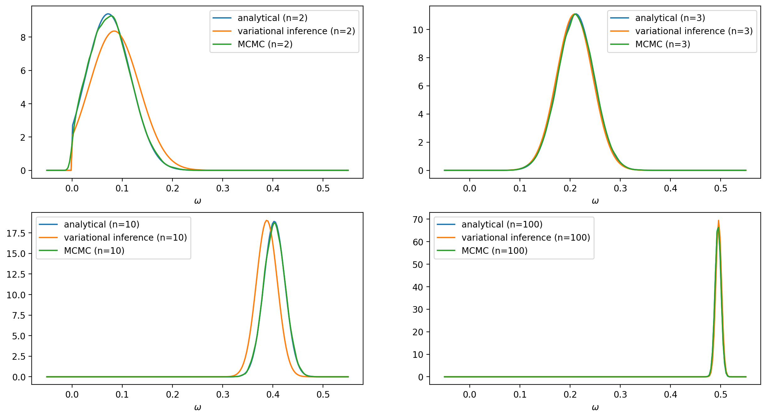
To solve the problem numerically we will use the TensorFlow Probability variational inference module. We will experiment with two different variational posteriors: the Log-normal and the Truncated normal distributions. The latter will be a better fit since it has exactly the same form as the exact solution. The data points that will be used to train the model are generated from the following equation: \begin{align*} y^{(j)} & = \omega \, x^{(j)} + \varepsilon^{(j)}, \hspace{4.0mm} \omega = .5, \hspace{1.0mm} \varepsilon \sim \mathcal{N}(0, \sigma=4) \end{align*} To see clearly the impact of the prior on the predictions we have chosen a rather high value $\lambda = 200$ for the rate $\lambda$ in \eqref{eq:prior}. We will compare the results obtained from the analytical, the variational inference, and the MCMC approach for a different number of data points. The complete source code can be found here.
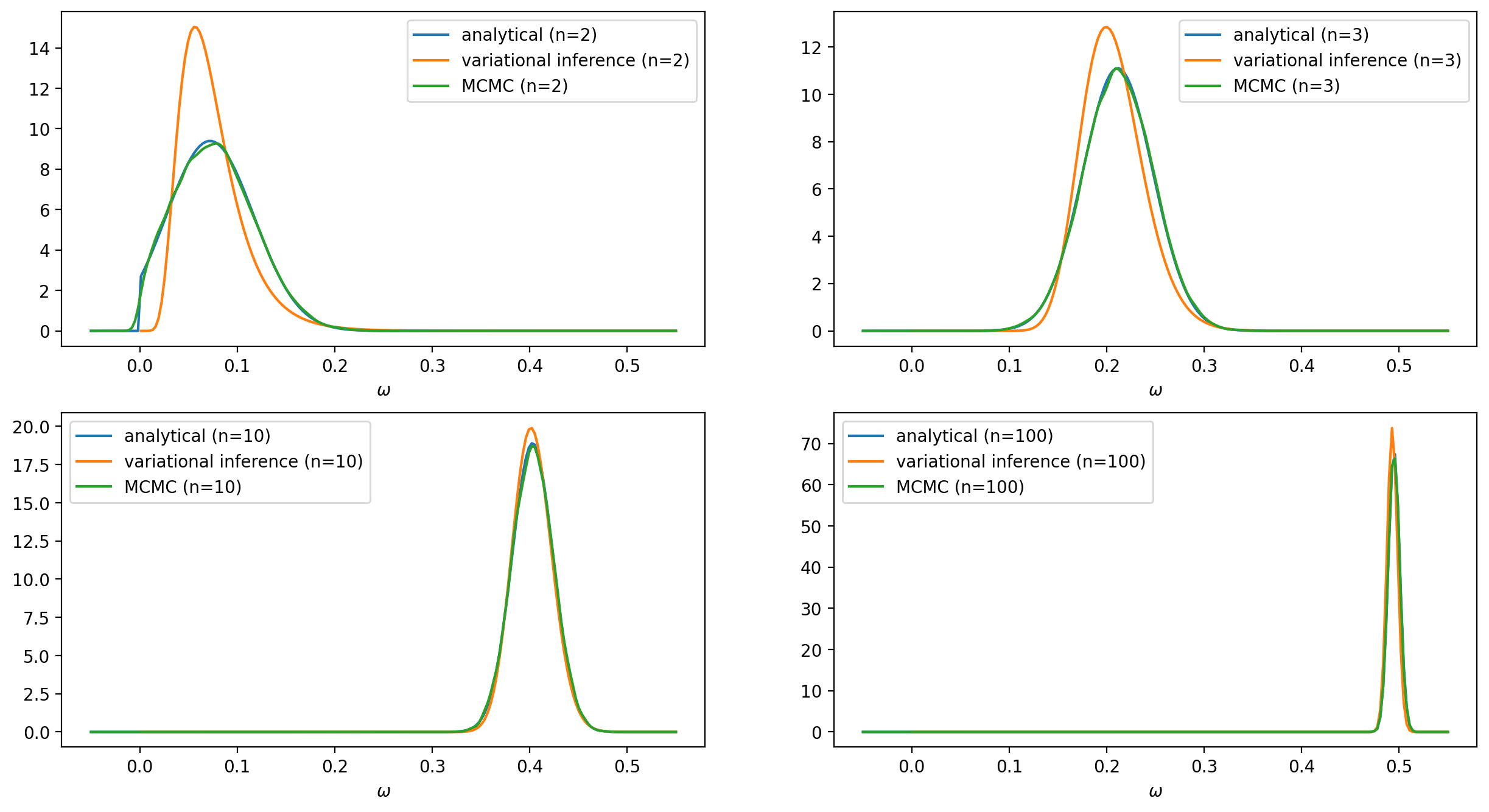
In the case of using a Log-normal distribution as a surrogate posterior, we cannot get as good results as those with the previous surrogate posterior. Nevertheless, the distribution $q$ still manages to follow the evolution of the mean and the standard deviation of the posterior $p(\omega |Y, X)$.
3. Final remarks
In the current example, we have only estimated the growth rate $\omega$, but we can extend both numerical approaches to estimate the standard deviation $\sigma$. Moreover, the case where there are multiple correlated height measurements of the same tree can be properly accounted for by the Tensorflow STS library, which could be demonstrated in a future post.
4. Ressources
- [1] Source code