Ad auction bidding strategy

Real-Time Bidding (RTB) has become a relevant paradigm in display advertising. It mimics stock exchanges and utilizes computer algorithms to buy and sell ads in real-time automatically. Imagine that you have to participate in $N \gg 1$ of those online ad auctions with a limited bidding budget. The task is to create such a bidding strategy that you can win some of them, and that the placed ads generate at least $N_C$ clicks. That should be done by spending as little money as possible. In the following, we will look at a possible solution to this problem.

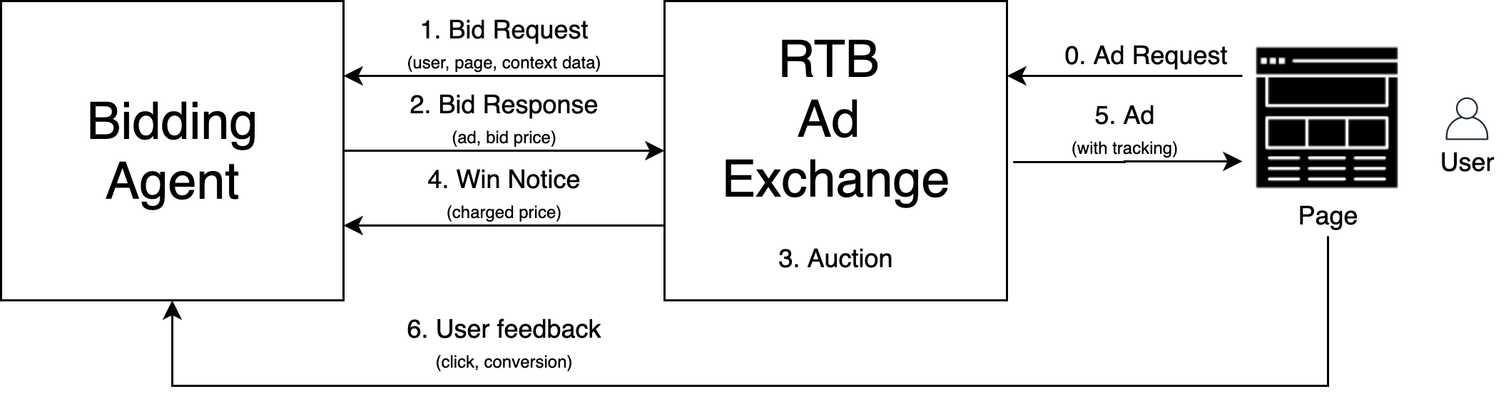
1. Real-Time Bidding ecosystem

A brief description of the RTB ecosystem is given in the figure above. When a user visits an ad-supported site each ad placement will trigger an auction. Bid requests will be sent via the ad exchange to the different bidding agents. Upon receiving a bid request, every bidding agent calculates a bid that is sent together with an ad to the Ad exchange. Finally, the winner’s ad will be shown to the visitor along with the regular content of the website. The whole process should be completed within a fraction of the second. A more detailed introduction to RTB could be found in [1,2].

2. Problem description

For simplicity, we will consider that we only have to create a strategy for a particular ad (for example, white sneakers from a particular brand) but the approach can be easily generalized to multiple ads, each one of them having a different budget and target. The ad exchange generates a large number of bid requests which are processed by many bidding agents, each one of them having the opportunity to make a bid. The user and publisher data contained in every bid request could be used to predict the probability distribution function of the winning bid price $s$, and the probability that the user will click on the displayed ad. For every auction $n \in \{1, \ldots N\}$ they will be denoted as: \begin{align} p_{C_n} & {\rm \hspace{4mm} click-through \hspace{0.7 mm} probability}\\ p_{S_n}(s) & {\rm \hspace{4mm} probability \hspace{0.7mm} distribution \hspace{0.7mm} function \hspace{0.7mm} of \hspace{0.7mm} the \hspace{0.7mm} winning \hspace{0.7mm} bid \hspace{0.7mm} price} \end{align} For every auction $n$, we will place a bid price $x_n$. The probability to win is then given by: \begin{align} p_{W_n| x_n} (x_n) & = \int^{x_n}_{0} p_{S_n}(s) ds. \end{align} The integral from $0$ to xn takes into account all cases where the winning bid price generated by taking into account all other participants except us is smaller than our bid price $x_n$. Because of the probabilistic nature of our assumptions, we can not guarantee which auction we are going to win or if a user will click on the displayed ad. To describe these random events we will use the following Bernoulli random variables: \begin{align} C_n & \sim {\rm Bernoulli}(p_{C_n}), \\ W_n| x_n & \sim {\rm Bernoulli}(p_{W_n|x_n} (x_n)), \end{align} where $C_n$ describes the user ad click events (click: $C_n=1$, no click: $C_n=0$) and $W_n|x_n$ — the event of winning the $n$-th auction by placing the bid price $x_n$ (win: $W_n|x_n=1$, loss: $W_n|x_n=0$). The probability for each one of these events to occur is given by: \begin{align*} \Pr (C_n =1) & = p_{C_n}, \\ \Pr (W_n | x_n =1) & = p_{W_n | x_n} (x_n) \end{align*} The total number user clicks on our ad obtained by placing the bids $ \{ x_n | n = 1, 2 \ldots N \} $ is given by: \begin{align} \Upsilon & = \sum\limits^{N}_{n=1} C_n \cdot W_n| x_n. \end{align} This is a random variable, as well. For simplicity, we will look only at its expected value: \begin{align} \mathbb{E} (\Upsilon) & = \sum\limits^{N}_{n=1} \mathbb{E} (C_n \cdot W_n| x_n) \nonumber \\ & = \sum\limits^{N}_{n=1} \mathbb{E} (C_n ) \cdot \mathbb{E} ( W_n| x_n) \nonumber \\ & = \sum\limits^{N}_{n=1} p_{C_n} \cdot p_{W_n| x_n} (x_n). \end{align} The amount of money spent on the auctions that we have won can be described by the following random variable: \begin{align} M & = \sum\limits^{N}_{n=1} x_n \cdot W_n|x_n. \end{align} As in the equation for the total number of click events, we will look only at the expected value of this variable: \begin{align} \mathbb{E} (M) & = \sum\limits^{N}_{n=1} x_n \cdot \mathbb{E} (W_n|x_n) \nonumber \\ & = \sum\limits^{N}_{n=1} x_n \cdot p_{W_n|x_n} (x_n) \end{align} The problem of placing $N$ bids $x_1, \ldots x_N$ such that the expected number of user clicks $\mathbb{E}(\Upsilon) = N_c $ and that the spent amount of money on winning bids is minimized can be solved with the method of the Lagrange multipliers: \begin{align} \mathcal{L}(x, \lambda) & = f(x) - \lambda g(x), \nonumber \\ f(x) & = \sum\limits^{N}_{n=1} x_n \cdot p_{W_n|x_n} (x_n), \nonumber \\ g(x) & = \sum\limits^{N}_{n=1} p_{C_n} \cdot p_{W_n| x_n} (x_n) - N_C, \label{eq:lagrange_multipliers} \end{align} where $f(x)$ has to be minimized under the condition that $g(x) = 0$.

3. Solutions to the optimization problem

We will consider an analytically solvable case that can be used to check if our numerical solution is implemented correctly. Then we will briefly describe some of the problems that arise if we apply this approach to real data: the large system of equations that have to be solved and the approximation of the winning bid probability distribution by using a finite number of observations. A numerical approach that addresses these two problems can be found in this Github repository.

3.1 Single click-through probability and winning bid distribution

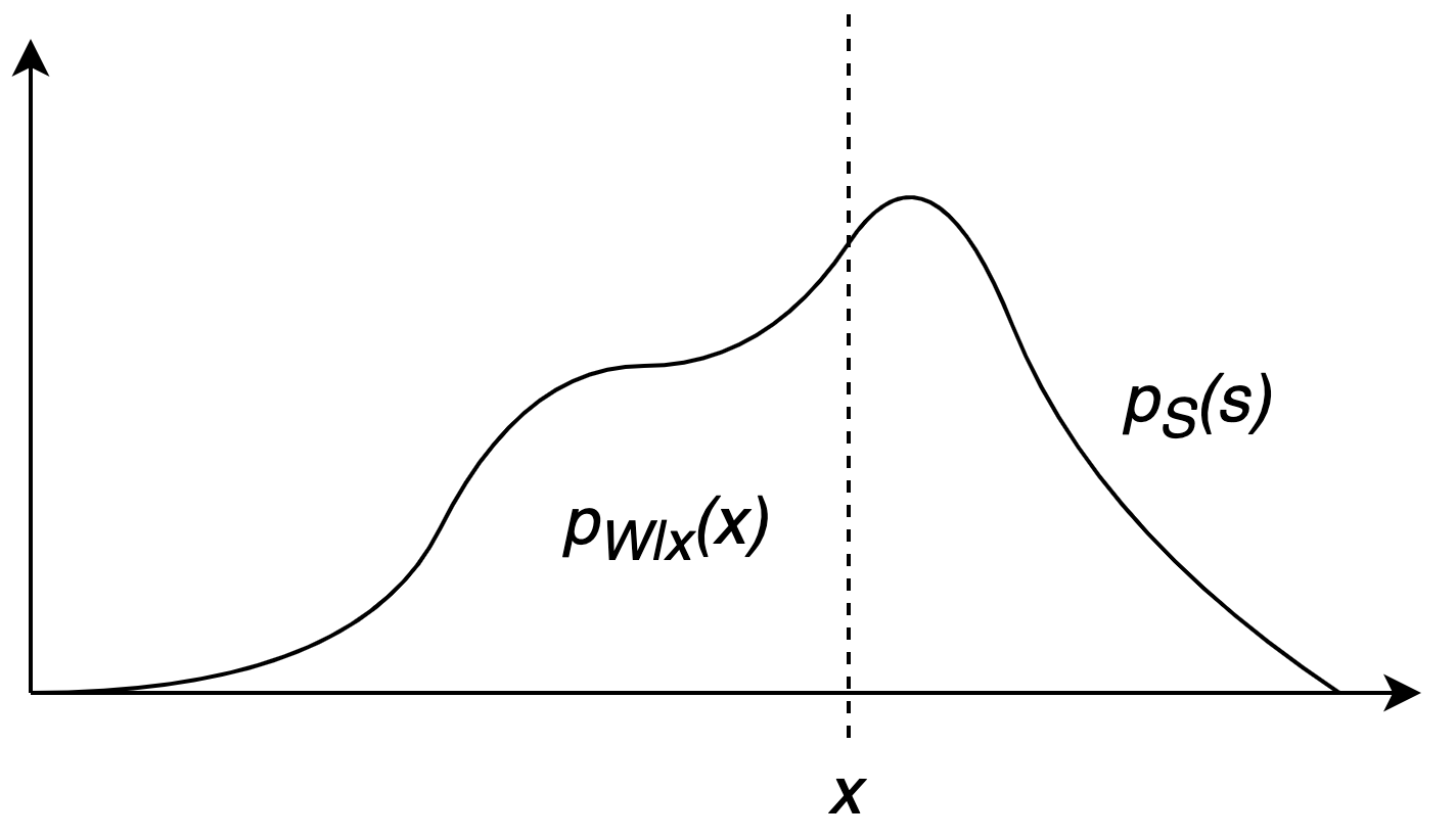
We will assume that the winning bid distribution for every auction n can be parametrized by an exponential distribution: \begin{align} p_{S_n}(s) & = \alpha_n e^{-\alpha_n s} \hspace{4.0mm} \alpha_n > 0. \end{align} It follows that the probability to win auction $n$ if our bid is $x_n$ is given by: \begin{align} p_{W_n | x_n} (x_n) & = \int^{x_n}_{0} p_{S_n} (s) ds \nonumber \\ & = \int^{x_n}_{0} \alpha_n e^{-\alpha_n s} ds \nonumber \\ & = 1 - e^{-\alpha_n x_n}. \end{align} To make the problem analytically solvable we have assumed that the probability distribution functions to win the auctions $1, \ldots N$ and the corresponding user click-through probabilities are all the same: \begin{align} \alpha_n & = \alpha, & n\in \{ 1, \ldots N \} \\ p_{C_n} & = p_C & n\in \{ 1, \ldots N \}. \end{align} By applying the method of the Lagrange multipliers, we obtain the optimal bid price $x_n$ and the expected amount of money spent to be: \begin{align} x_n & = \frac{1}{\alpha} \ln \Big( \frac{N \cdot p_C}{ N \cdot p_C - N_C } \Big), \hspace{4.0mm} n\in \{ 1, \ldots N \} \\ \mathbb{E}(M) & = \frac{N_C}{p_C} \frac{1}{\alpha} \ln \Big( \frac{N \cdot p_C}{ N \cdot p_C - N_C } \Big). \end{align} In real situations, we expect that $N \cdot p_c \gg N_c$ (i.e. we have to win only a small fraction of all auctions to achieve the goal of getting $N_c$ clicks) which allows us to expand $\log ()$ around $1$: \begin{align} x_n & \approx \frac{1}{\alpha} \frac{N_C}{N \cdot p_C}, \\ \mathbb{E}(M) & \approx \frac{1}{\alpha}\frac{N^2_C}{N \cdot p^2_C} . \end{align} Since $1/\alpha$ is the mean value of the exponential distribution function and $N_c/(N \cdot p_c) \ll 1$, it follows that $x$ is a very low value, i.e. we are participating at every auction with a very low bid price. We may speculate that a similar result is obtained if we use different probability distribution functions for the prices of successful bids, i.e. that we will only be interested in the left side of the distribution because that is where the optimal value is located. This also implies that we should have a very precise description of $p_{W|x}$ for a small $x$, which in practice could be a difficult task to achieve.

3.2 Multiple click-through probabilities and winning bid distributions

The general case where each auction is described by a unique probability distribution function and where the click-through probabilities can be different for each $n$ can be solved numerically using the Python scipy library. This approach quickly becomes unfeasible if $N$ is in the order of $10^3$, which is not sufficient for more realistic cases with $N > 10^6$. To make the problem manageable by the python scipy library, we will assume that the winning bid distribution of an auction can be described by one out of $I$ different possible probability distribution functions: \begin{align} \tilde{p}_{S_i}(s) \hspace{5.0mm} i \in \{1, 2, \ldots I \}. \end{align} The same idea can be applied to the click-through probability which can only take $J$ different values: \begin{align} \tilde{p}_{C_j} \hspace{5.0mm} j \in \{1, 2, \ldots J \}. \end{align} If we look closely at the solution to the optimization problem \eqref{eq:lagrange_multipliers}, we see that the optimal bid price is the same for all auctions with the same distribution of successful bids $i$ and the same click-through probability $j$. We will denote this optimal price with $\tilde{x}_{ij}$. With these considerations in mind, the functions $f$, $g$ from the Lagrange optimization problem \eqref{eq:lagrange_multipliers} can be rewritten to: \begin{align} f(\tilde{x}) & = \sum\limits^{I}_{i=1} \sum\limits^{J}_{j=1} N_{ij} \cdot \tilde{x}_{ij} \cdot \tilde{p}_{W_i|\tilde{x}_{ij}} (\tilde{x}_{ij}) , \\ g(\tilde{x}) & = \sum\limits^{I}_{i=1} \sum\limits^{J}_{j=1} N_{ij} \cdot \tilde{p}_{C_j} \cdot \tilde{p}_{W_i|\tilde{x}_{ij}} (\tilde{x}_{ij}) - N_C, \end{align} where $N_{ij}$ is equal to the number of cases where the distribution of successful bids is of type $i$ and the click-through probability is of type $j$. With this simplification, we can numerically solve problems where $I·J <10^3$.

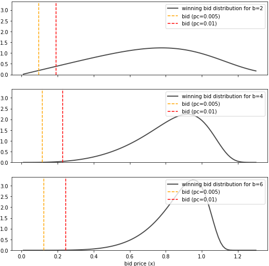
To demonstrate the applicability of this approach, we have considered the case where $I=3$ and $J=2$: \begin{align} \tilde{p}_{C_1} & = 0.005, \nonumber \\ \tilde{p}_{C_2} & = 0.01, \nonumber \\ \tilde{p}_{S_i} (s) & = b_i s^{b_i-1} \exp \big(1 +s^{b_i} - \exp(s^{b_i}) \big) \hspace{5.0mm} b_1 =2, \hspace{1.0mm} b_2 =4, \hspace{1.0mm} b_3=6. \end{align} The optimal solution is shown in the following figure:

3.3 Obtain probability distribution functions from real data

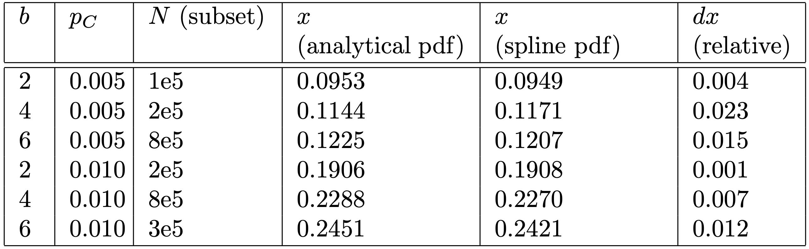
Under realistic conditions, we have to infer the probability distribution of successful bids from the events (prices of successful bids) in our data. We can count the number of events for a grid of $x$ values and then use spline interpolation as an approximation of the distribution function. We have applied this idea to the previous example, where instead of using the analytical form of the winning bid distribution, we have sampled data points from this distribution. From the table above you can see that the differences between the two solutions are minimal. We must take into account that the number of sampled data points per distribution is in the order of $10^6$. A lower number of sampled data points inevitably leads to a lower accuracy of the spline approximation. We also have to keep in mind that the spline approximation generates a function $h(x)$ whose second derivative $d^2h(x)/dx^2$ is zero at the boundaries of the $x$ grid. This restriction can become problematic for probability distribution functions that do not go to $0$ for $x \rightarrow 0$. One such example is the exponential probability distribution function, where the second derivative at $x = 0$ is: \begin{align} \frac{d^2}{dx^2} \alpha e^{-\alpha x} \Big\vert_{x=0} & = \alpha^3 > 0. \end{align} Another problem is that with the spline approximation we cannot guarantee that the resulting function is non-negative.

Summary

In this article, we have created a simple bidding strategy by assuming that we know the winning bid probability distribution function of each auction and the click-through probability for each advertising event. From the two examples we have considered, we have seen that the optimal solution requires precise knowledge of the left side of the winning bid probability distribution function.

Resources

• [1] Real-Time Bidding Benchmarking with iPinYou Dataset
• [2] Real-time Bidding for Online Advertising: Measurement and Analysis
• [3] Source code