
Federated learning is a machine learning technique that trains a model across multiple decentralized devices, each of them holding a local data sample, without exchanging these data samples. Let’s imagine that by using this technique you have trained a binary classification model. You want to test it on the data of several devices by calculating the model ROC-AUC score on each one of them and then by averaging the results. The following questions arise:
- How much does this score differ from the ROC-AUC score that could have been obtained if all the data was located on the same device?
- Under which conditions are both scores equal? Are they equal only in the case when the data is identically distributed among all devices?
Motivation: Federated learning
Compared to the centralized learning approach where the data is stored on a single server and we have constant access to it during training, in the federated learning setting the data is held by multiple devices that can participate at different times in the training process without sharing their data. A possible federated training procedure is composed of the following steps which are repeated multiple times until the model is trained:
- send the model to every active device that is willing to participate in the training process;
- for every device train a model on a single data batch of the corresponding device;
- return the trained model weights to the central server where the model weights are aggregated in a secure way such that the server is not aware of the contributions of the different devices to the averaged model weights;
- check the model performance on a validation data set and decide if you should stop the training process;
In this setting, the central server receives only the averaged model weights updates from all devices, which in combination with other privacy-preserving methods hinders him to guess how the data in the different devices, for example, mobile phones, looks like.
If we want to check the model performance, we would like to do this in a way that we can gather as little information about the data as possible. A possible solution could be to calculate a model performance metric $A$ (like the ROC-AUC score) in every device for the data contained in this device and then to send the securely calculated average of the metrics to the server. In this case, the model owner (server) receives this averaged metric but does not know how it relates to the metric $A(D)$ calculated if all the data $D$ was in one place, i.e. he does not know if:
$$ \begin{align} \label{eq:roc_auc_inequality} A_{roc} ( D ) & \stackrel{?}{=} \frac{1}{M} \sum\limits^{M}_{m=1} A_{roc}(D_m), \\ D & = \bigcup\limits^{M}_{m=1} D_m, \nonumber \end{align} $$ where we have split the data $D$ into $M$ subsets.ROC-AUC definition
We will consider the case of having a binary classification problem. A data set composed of features $(x \in \mathbb{R}^n)$ and target values $(y \in \{0, 1\} )$ is used to train a model $g: \mathbb{R}^n \rightarrow \mathbb{R} $ that assigns to every feature a score $\xi = g(x)$. By comparing the score $\xi$ with a threshold $T$ we can decide if a given element belongs to the class $y=1$ (when $\xi > T$) or to the class $y=0$ (otherwise).
For example, we can consider the case of having a data set with three features $(x \in \mathbb{R}^3)$, target variable $y$ and a model $g$ that is defined as follows: $$ \begin{align} g: \mathbb{R}^3 & \rightarrow \mathbb{R} \nonumber \\ x & \mapsto g(x) = \omega_0 + \omega_1 \cdot x_1 + \omega_2 \cdot x_2 + \omega_3 \cdot x_3, \end{align} $$ where the $\omega_0, \omega_1, \omega_2, \omega_3$ denote the trained parameters of the model.
We can separate the calculated scores $\xi$ in two groups: a group of scores obtained from data points that belong to the positive class $(y=1)$ and to the negative class $(y=0)$, respectively. Both groups of scores can be interpreted as samples from probability distribution functions $f_{+}, f_{-}$ for the elements of the first and second groups, respectively. A sample visualization of both distributions is given in the figure below.
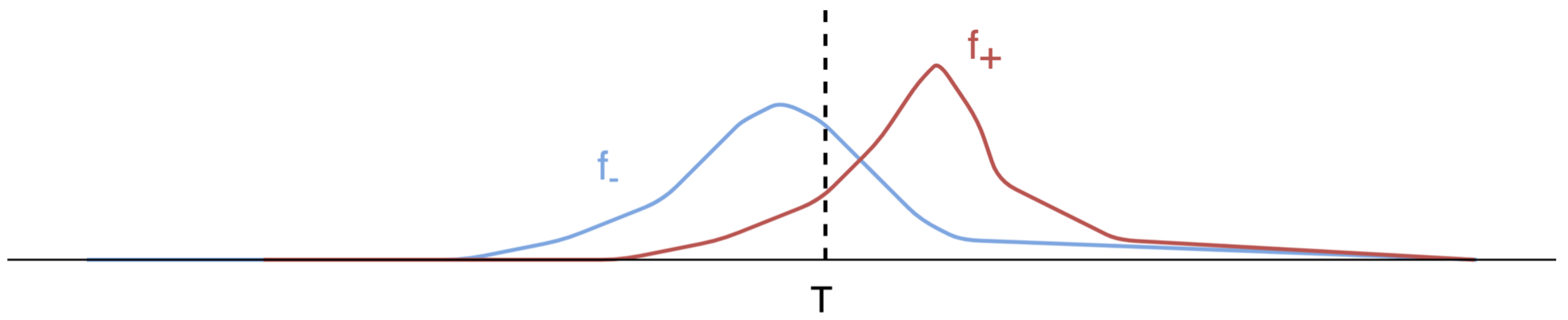
The figure represents a common case where we are not able to set the threshold $T$ such that both probability distribution functions can be completely separated. Some of the members of the negative class are classified as positive (False positive = FP; this is the area under the blue curve on the right side of $T$) and some members of the positive class are classified as negative (False negative = FN; this is the area under the red curve on the left side of $T$). In general, the better the model the smaller the overlap between $f_{+}, f_{-}$ and with it the smaller the number of false positives and false negatives.
The area of $f_{-}, f_{+}$ on the right side of $T$ is equal to the false positive rate (FPR), and to the true positive rate (TPR) respectively. Both are defined as: $$ \begin{align} {\rm FPR} (T) & = \frac{ {\rm FP} (T)}{N} = \int^{\infty }_{T} f_{-} (\xi) d\xi, & \int^{\infty }_{-\infty} f_{-} (\xi) d\xi & = 1 \\ {\rm TPR} (T) & = \frac{ {\rm TP} (T)}{P} = \int^{\infty }_{T} f_{+} (\xi) d\xi, & \int^{\infty }_{-\infty} f_{+} (\xi) d\xi & = 1 \end{align} $$
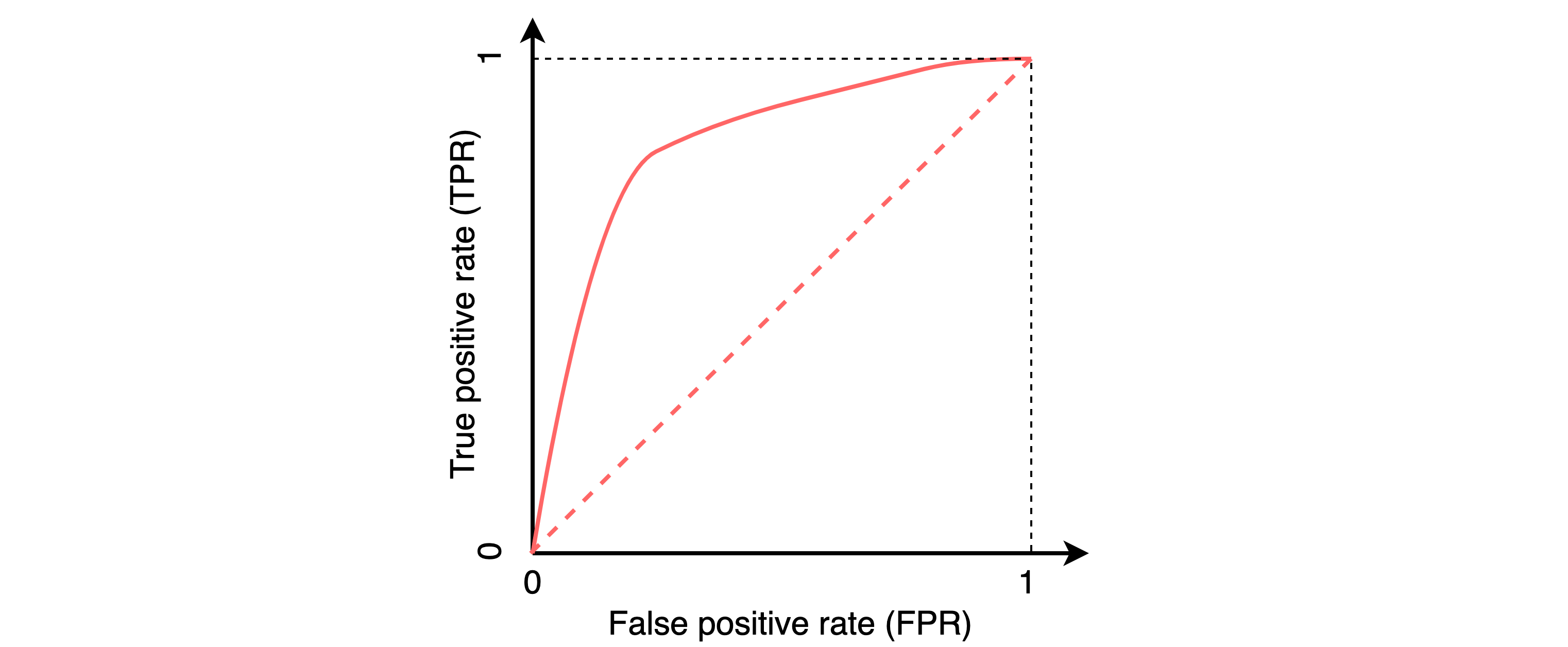
The receiver operating characteristic curve, or ROC curve, is a graphical plot that illustrates the ability of a model to discriminate between two classes as its discrimination threshold T is varied. The ROC-AUC score is defined as the area under the ROC curve and it is used to measure the model performance. This score can be expressed as a function of both probability distribution functions f₊, f₋, as follows: $$ \begin{align} \label{eq:roc-auc-def} A_{roc} & =\int^{1}_{0} {\rm TPR}\big( {\rm FPR}^{-1} (x) \big) dx = \int^{-\infty}_{\infty} {\rm TPR} (\xi) {\rm FPR}' (\xi) d\xi, \end{align} $$ where ${\rm FPR}'(\xi)$ refers to the derivative of ${\rm FPR}(\xi)$ with respect to $\xi$. This equation will be used to explain some of the differences between the ROC-AUC score and the proposed averaged ROC-AUC score in federated learning mode.
ROC-AUC in the federated learning mode
As already mentioned in the Motivation: Federated learning section, we will look at \eqref{eq:roc_auc_inequality} for the case where the metric $A$ is equal to the ROC-AUC score, i.e:
$$ \begin{align} \label{eq:roc_auc_inequality_again_a} A_{roc} ( D ) & \stackrel{?}{=} \frac{1}{M} \sum\limits^{M}_{m=1} A_{roc}(D_m), \\ \label{eq:roc_auc_inequality_again_b} D & = \bigcup\limits^{M}_{m=1} D_m, \end{align} $$The number of devices is $M$ and $D_m$ denotes the data contained in the $m$-th device. In the following sections, we will see that the equality in \eqref{eq:roc_auc_inequality_again_a} depends on the distribution functions $(f_{+}, f_{-})$ of the scores for each device. We will consider several cases.
Case 1: the $f_{+}, f_{-}$ distributions among the devices are identical
To warm-up, we will consider the trivial case where the data points contained in every one of the $M$ devices are identically distributed. This means that the distributions $f_{+m}, f_{-m}$ $(m = 1, 2, \ldots M)$ of the scores obtained from applying the trained model to the data on each one of the $M$ devices are the same, i.e.:
$$
\begin{align}
f_{+m} (\xi) & = f_{+} (\xi) , & f_{-m} (\xi) & = f_{-} (\xi) \hspace{6.0mm} m = 1, 2, \ldots M.
\nonumber
\end{align}
$$
The same statement can be applied to the false positive $({\rm FPR}_m)$ and to the true positive $({\rm TPR}_m)$ rates which are derived from $f_{-}$ and $f_{+}$, respectively. By using \eqref{eq:roc-auc-def} we can conclude that the ROC-AUC score for each one of the $M$ devices will be the same, i.e.:
$$
\begin{align}
A_{roc,m} & = \int^{-\infty}_{\infty} {\rm TPR}_m (\xi) {\rm FPR}'_m (\xi) d\xi \nonumber \\
& = \int^{-\infty}_{\infty} {\rm TPR} (\xi) {\rm FPR}' (\xi) d\xi = A_{roc}
\hspace{12.0mm} m = 1, \ldots M.
\label{eq:roc-auc-equiv-dist}
\end{align}
$$
It follows that the average ROC-AUC score across all devices is equal to the ROC-AUC score for the entire data set.
$$
\begin{align}
\label{eq:A_roc_equality}
\frac{1}{M} \sum\limits^{M}_{m=1} A_{roc,m} & \stackrel{\eqref{eq:roc-auc-equiv-dist}}{=}
\frac{1}{M} \sum\limits^{M}_{m=1} A_{roc} = A_{roc}.
\end{align}
$$
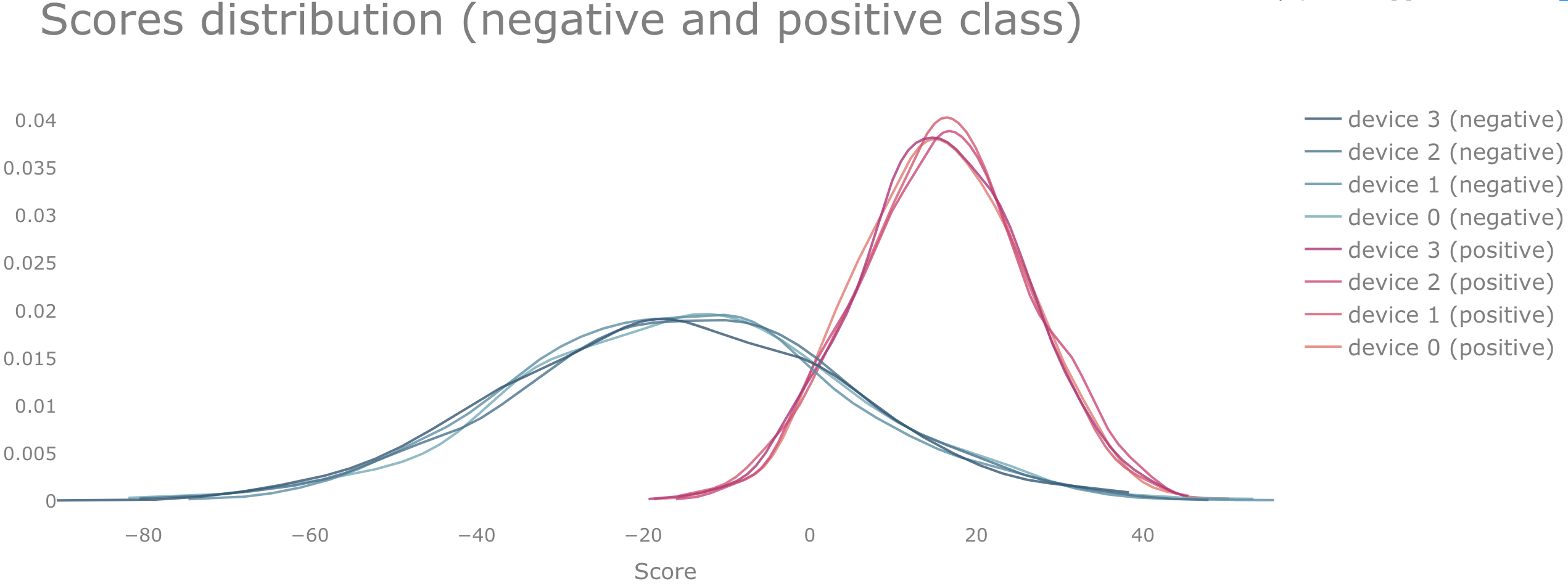
For example, we can consider the case of having 4 devices, each of them having 500 elements of the positive and 500 elements of the negative class, respectively (the source code used to generate this example is provided at the end of the post). The elements are split between the devices such that the distributions of the scores
$$
\begin{align}
f_{-,m} & \sim \mathcal{N} (\mu_-, \sigma^2_{-}), \nonumber \\
f_{+,m} & \sim \mathcal{N} (\mu_+, \sigma^2_{+}), \hspace{6.0mm} m = 1,2,3,4 \nonumber \\
\mu_- = -16, & \hspace{4.0mm} \mu_+ = 16, \hspace{4.0mm}
\sigma_- = 20, \hspace{4.0mm} \sigma_+ = 10 \nonumber
\end{align}
$$
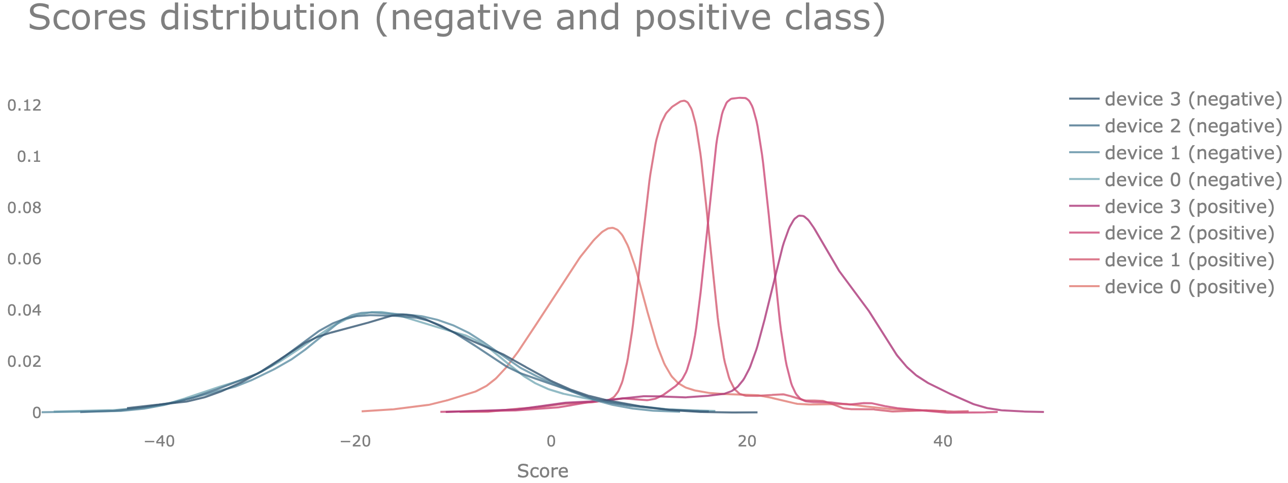
are approximately the same and normally distributed with mean $\mu_{-}, \mu_{+}$, and standard deviation $\sigma_{-}$, $\sigma_{+}$, as shown in the figure below. Such a situation can be achieved if the data is identically distributed among all devices.
Case 2: the $f_{+}$, $f_{-}$ distributions among the devices are not identical
If we consider the case where the data points contained in every one of the $M$ devices are not identically distributed, we can represent $f_{+}$ and $f_{-}$ as follows: $$ \begin{align} \label{eq:fmin_fmin-m__equivalence} f_{-} (\xi) & = \sum\limits^{M}_{m=1} \frac{I_{-m}}{ I_- } f_{-,m} (\xi), \\ \label{eq:fplu_fplu-m__equivalence} f_{+} (\xi) & = \sum\limits^{M}_{m=1} \frac{I_{+m}}{ I_+ } f_{+,m} (\xi), \end{align} $$ where $I_{-}$, $I_{+}$ refer to the number of points of the positive/negative class in the entire data set, and $I_{-m}$, $I_{+m}$ to the corresponding number in the $m$-th device, respectively. It follows that: $$ \begin{align} \label{eq:fpr_fprm_relation} {\rm FPR} (T) & = \int^{\infty }_{T} f_{-} (\xi) d\xi \stackrel{\eqref{eq:fmin_fmin-m__equivalence}}{=} \sum\limits^{M}_{m=1} \frac{I_{-,m}}{I_-} \int^{\infty }_{T} f_{-,m} (\xi) d\xi = \sum\limits^{M}_{m=1} \frac{I_{-,m}}{I_-} {\rm FPR} _m(T), \\ \label{eq:tpr_tprm_relation} {\rm TPR} (T) & = \int^{\infty }_{T} f_{+} (\xi) d\xi \stackrel{\eqref{eq:fplu_fplu-m__equivalence}}{=} \sum\limits^{M}_{m=1} \frac{I_{+,m}}{I_+} \int^{\infty }_{T} f_{+,m} (\xi) d\xi = \sum\limits^{M}_{m=1} \frac{I_{+,m}}{I_+} {\rm TPR} _m(T). \end{align} $$
Case 2.1: only the $f_{-}$ distributions among the devices are identical
This has the following implication: $$ \begin{align} \label{eq:fpr_fprm_equivalence_1} {\rm FPR}_m (T) & = \int^{\infty}_{T} f_{-,m} (\xi) d\xi = \int^{\infty}_{T} f_{-} (\xi) d\xi = {\rm FPR} (T) , \\ \label{eq:fpr_fprm_equivalence_2} \Rightarrow {\rm FPR}'_m (T) & = {\rm FPR}' (T), \end{align} $$ where ${\rm FPR}'(T) = d {\rm FPR}(T)/dT$ . The weighted average ROC-AUC score across all devices is then given by: $$ \begin{align} \sum \limits^{M}_{m=1} \frac{I_{+,m}}{I_+} A_{roc,m} & \hspace{2mm} = \hspace{2mm} \sum \limits^{M}_{m=1} \frac{I_{+,m}}{I_+} \int^{\infty}_{-\infty} {\rm TPR}_m (\xi) \cdot {\rm FPR}'_m (\xi) d\xi \nonumber \\ & \hspace{0.97mm} \stackrel{\eqref{eq:fpr_fprm_equivalence_2}}{=} \hspace{1mm} \sum \limits^{M}_{m=1} \frac{I_{+,m}}{I_+} \int^{\infty}_{-\infty} {\rm TPR}_m (\xi) \cdot {\rm FPR}' (\xi) d\xi \nonumber \\ & \hspace{2mm} = \hspace{2mm} \int^{\infty}_{-\infty} \sum \limits^{M}_{m=1} \frac{I_{+,m}}{I_+} {\rm TPR}_m (\xi) \cdot {\rm FPR}' (\xi) d\xi \nonumber \\ & \stackrel{\eqref{eq:tpr_tprm_relation}}{=} \int^{\infty}_{-\infty} {\rm TPR} (\xi) \cdot {\rm FPR}' (\xi) d\xi \nonumber \\ & \hspace{2mm} = \hspace{2mm} A_{roc}, \label{eq:fpr_fprm_equivalence_proof} \end{align} $$ i.e. it is equal to the ROC-AUC score of the entire data set. If the number of elements from the positive class from every device $I_{+m}$ is the same, the last equation reduces to \eqref{eq:A_roc_equality}.
To illustrate this we can use again the same example with 4 devices that we have used in the previous section. We use the same data which in this case is distributed among the devices in a way that only the data points belonging to the negative class are identically distributed among all devices.
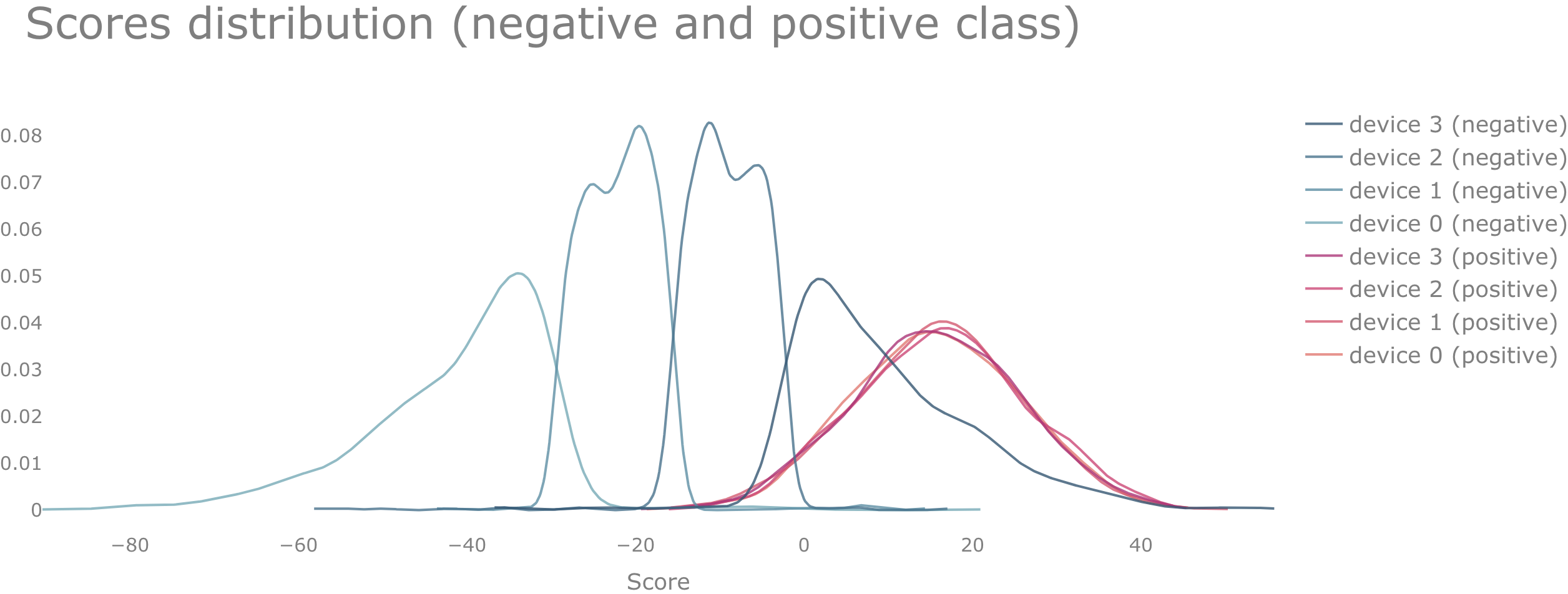
Case 2.2: only the f₊ distributions among the devices are identical
This has the following implication: $$ \begin{align} \label{eq:tpr_tprm_equivalence_1} {\rm TPR}_m (T) & = \int^{\infty}_{T} f_{+,m} (\xi) d\xi = \int^{\infty}_{T} f_{+} (\xi) d\xi = {\rm TPR} (T). \end{align} $$ We can use equation \eqref{eq:tpr_tprm_equivalence_1} in the same way as \eqref{eq:fpr_fprm_equivalence_2} was used to prove \eqref{eq:fpr_fprm_equivalence_proof}: $$ \begin{align} \label{eq:tpr_tprm_equivalence_proof} \sum \limits^{M}_{m=1} \frac{I_{-,m} }{I_-} A_{roc,m} & \hspace{2mm} = \hspace{2mm} \sum \limits^{M}_{m=1} \frac{I_{-,m} }{I_-} \int^{\infty}_{-\infty} {\rm TPR}_m (\xi) \cdot {\rm FPR}'_m (\xi) \hspace{0.5mm} d\xi \nonumber \\ & \hspace{0.97mm} \stackrel{\eqref{eq:tpr_tprm_equivalence_1}}{=} \hspace{1mm} \sum \limits^{M}_{m=1} \frac{I_{-,m} }{I_-} \int^{\infty}_{-\infty} {\rm TPR} (\xi) \cdot {\rm FPR}'_m (\xi) \hspace{0.5mm} d\xi \nonumber \\ & \hspace{2mm} = \hspace{2mm} \int^{\infty}_{-\infty} {\rm TPR} (\xi) \cdot \frac{I_{-,m}}{I_-} \sum \limits^{M}_{m=1} {\rm FPR}'_m (\xi) \hspace{0.5mm} d\xi \nonumber \\ & \stackrel{\eqref{eq:fpr_fprm_relation}}{=} \int^{\infty}_{-\infty} {\rm TPR} (\xi) \cdot {\rm FPR}' (\xi) \hspace{0.5mm} d\xi \nonumber \\ & \hspace{2mm} = \hspace{2mm} A_{roc}. \end{align} $$ In the case of having the same number of elements from the positive class $I_{+m}$ in every device, this equation reduces to \eqref{eq:A_roc_equality}, i.e. the average ROC-AUC score is again equal to the ROC-AUC score of the entire data set.
To illustrate this, we can use again the same example with 4 devices that we have used in the previous section. We use the same data which in this case is distributed among the devices in a way that only the data points belonging to the positive class are identically distributed among all devices.
Case 2.3: Neither the $f_{+}$ nor the $f_{-}$ distributions among the devices are identical
In this case, we cannot expect that equation \eqref{eq:A_roc_equality} will be fulfilled. In our numerical example, we indeed see that both sides of \eqref{eq:A_roc_equality} are not equal if $f_{+}$ and $f_{-}$ are different among the devices.
Summary
In this article, we have looked at how a weighted average of ROC-AUC scores among multiple devices, each of them holding a local data set, changes in comparison to the case of calculating the ROC-AUC score of the complete data set on a single device. A sufficient condition for equivalence of both metrics is that either the distribution of the positive or of the negative scores among all devices is identical.
This work was done within the scope of the polypoly project.