We will look at the problem of navigating through a dynamically changing map. It can be represented as a sequence of optimization problems for every time step and in the end, it will reduce to a specific case of the Bellman equation. A solution will be discussed and applied to a particular realization of the problem.

We will consider a map with impenetrable (dynamic) obstacles like the moving brick walls, the cactus or the animal bones, and points through which you can pass but it is not preferable to do so (the blue monster). The goal is to reach the treasure as fast as possible.
Definition of a path
To navigate successfully through a map like the one in the figure above for a time period $ [0, T] $ we have to find a set of policies \( \{ \pi_t | t = 0, \ldots T-1 \} \) that will tell us in which direction to move given the time and our position in the map. A possible journey can be described by the sequence of points \( s_0, s_1, \ldots, s_T \) and the corresponding probability to use this sequence is given by: $$ \begin{align} P ( s_{T}, s_{T-1}, \ldots, s_0 ) = & P ( s_{T} | s_{T-1}, \ldots, s_0 ) \cdot \label{eq:traj_prob} \\ & P ( s_{T-1} | s_{T-2}, \ldots, s_0 ) \cdot \nonumber \\ & \ldots \nonumber \\ & P ( s_{1} | s_{0} ) \cdot \nonumber \\ & P ( s_{0} ). \nonumber \end{align} $$
The conditional probability density function \( P( s_{t+1}|s_t, \ldots s_0) \) describes the probability to move to \( s_{t+1} \) given the history of previously visited points \( s_t, … s_0 \). This probability depends on the map (if a point \( s_{t+1} \) is an obstacle or not) and on the policy \( \pi_t \). We will consider the case that the decision to which point \( s_{t+1} \) to move depends only on the current position \( s_t \), i.e: $$ \begin{align} \label{eq:markov_assumption} P( s_{t+1} | s_t, \ldots, s_0 ) & = P_{\pi_{t}(\lambda (t,s_t) )} ( s_{t+1} | s_t ) \hspace{4.0mm} t = 0, 1, \ldots T-1, \end{align} $$ which is also known as the Markov assumption. To emphasize the dependency of \( P \) on the policy, in the last equation we have added \( \pi (\lambda) \) as a subscript where \( \lambda (t, s) \) is a column vector containing all parameters that have to be learned: $$ \begin{align} \lambda(t, s_t) = & [\lambda_0(t, s_t), \ldots, \lambda_4(t, s_t) ]^T. \label{eq:lam_vec_definition} \end{align} $$
Example: conditional probability density function
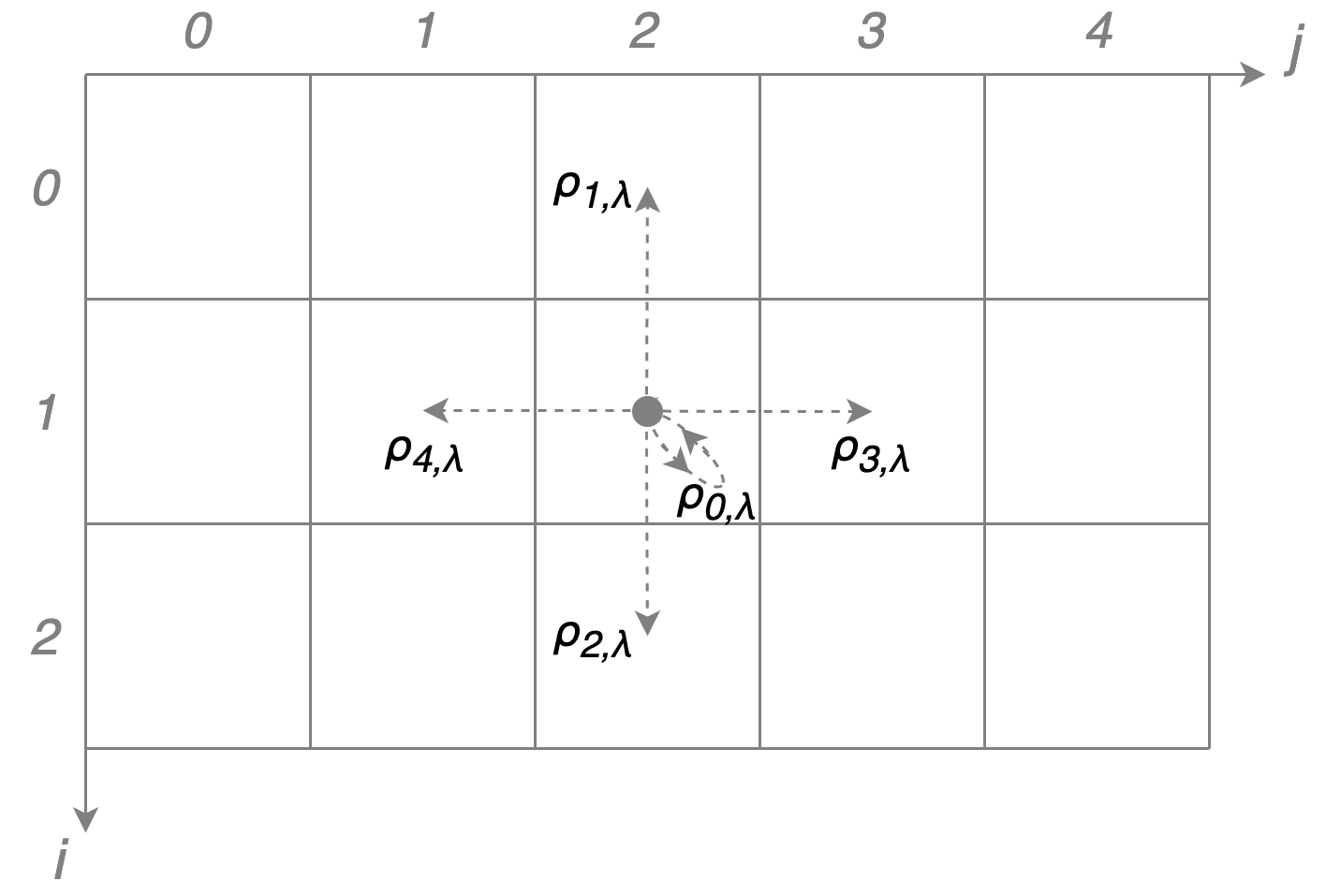
Let's give an example how $ P(s’|s) $ might look like. It makes sense to allow only movements towards the four closest bins (up, down, right, left) and to allow the possibility to stay idle. We represent the position s as a tuple $ (i, j) $ where $ i, j $ refer to the $i$-th row and $j$-th column of the sample map presented above. In this case the conditional probability density function is given by: $$ \begin{align} \label{eq:propagator_parametrization} P_{\pi_{t}(\lambda)} ( \underbrace{s_{t+1}}_{(i'j')} | \underbrace{s_t}_{(i,j)} ) & = \begin{array}{ll} & \delta_{i',i \textcolor{white}{-1} } \delta_{j',j\textcolor{white}{-1}} \rho_{0,\lambda} (t, s_t) + \\ & \delta_{i',i-1} \delta_{j',j\textcolor{white}{-1}} \rho_{1,\lambda} (t, s_t) + \\ & \delta_{i',i+1} \delta_{j',j\textcolor{white}{-1}} \rho_{2,\lambda} (t, s_t) + \\ & \delta_{i',i \textcolor{white}{-1} } \delta_{j',j+1} \rho_{3,\lambda} (t, s_t) + \\ & \delta_{i',i \textcolor{white}{-1} } \delta_{j',j-1} \rho_{4,\lambda} (t, s_t) , \end{array} \end{align} $$ where \( \delta \) is the Kronecker delta (it is equal to \( 1 \) if both subscripts are equal and \( 0 \) otherwise) and \( \rho_k(t, s) \) \( ( k=0,1,2,3,4) \) are the probabilities to stay \( (k=0) \) or move up \( (k=1) \), down \( (k=2) \), right \( (k=3) \), left \( (k=4) \) from the point \(s\) at time \(t\). An example is shown in the figure above. These probabilities have to sum up to \(1\) which naturally leads to the use of a softmax function for parametrization: $$ \begin{align} \label{eq:rho_parametrization} \rho_{k,\lambda} (t, s_t) = \frac{ e^{\lambda_k (t, s_t)} }{ \sum\limits^{4}_{\tilde{k}=0} e^{\lambda_{\tilde{k}} (t, s_t)} } \hspace{4.0mm} k=0,\ldots 4. \end{align} $$ The task of finding the most efficient set of policies is equivalent to finding \( \lambda_k(t, s) \) for all \(k\), \(t\), \(s\).
Define the best path
To find the best path we will assign a score to every path: we introduce rewards at the desired destination and penalties at the forbidden map points, summarized in the function \(R(t, s)\), which are added to the score of a path if we cross or stay at one of these points. The task is to maximize the collected score which can happen if we reach the destination as fast as possible and stay there in order to collect as many times the reward as possible.
The average score for a set of policies \( \{ \pi_t|t=0, .. T-1 \} \) under the condition that at \(t=0\) we are at position \(s_0\) is given by: $$ \begin{align} \label{eq:avg_score_for_some_policy} \sum\limits^{}_{s_T, \ldots, s_1} \sum\limits^{T-1}_{t=0} R(t+1, s_{t+1}) \underbrace{ \prod\limits^{T-1}_{\tau=0} P_{\pi_{\tau}(\lambda ) } ( s_{\tau+1} | s_{\tau} ) }_{ P(s_T, \ldots s_1| s_0)}. \end{align} $$ The first summation over \(s\) is responsible for the exploration of all possible trajectories, the second summation over \(t\), together with \(R\) defines the reward for a given trajectory, and the last term with underbrace represents the probability for a realization of a trajectory starting from \(s_0\). The reader can compare this term with equation \eqref{eq:traj_prob} and see that $$ \begin{align} P(s_T, \ldots s_1| s_0) & = P(s_T, \ldots s_0) / P(s_0), \end{align} $$ as expected. Our task is to define the policies such that the expected score is maximized: $$ \begin{align} \label{eq:avg_score_for_optimal_policy} V^*_{[T-1, \ldots , 0]} (s_0) & = _{ \pi_{T-1} , \ldots , \pi_0 }^{ \hspace{4.0mm} \rm max } \sum\limits^{}_{s_T, \ldots, s_1} \sum\limits^{T-1}_{t=0} R(t+1, s_{t+1}) \prod\limits^{T-1}_{\tau=0} P_{\pi_{\tau} (\lambda)} (s_{\tau+1} | s_{\tau}) . \end{align} $$ The indices in the square brackets in the left hand side refer to the policies \( \{ \pi_t|t=0, .. T-1\} \) that have to be optimized.
Example: reward/penalty function
The reward and penalties can be parametrized as follows: $$ \begin{align} \label{eq:reward_definition} R(t, s_t ) &= \delta_{i,0} \delta_{j,7} - 6 \delta_{i,1} \delta_{j,7} , \hspace{4.0mm} s_t \equiv (i,j). \end{align} $$ The first term corresponds to the reward that we get at every time step when we are in the upper right corner of the map and the second term corresponds to the penalty that we get when we stay one bin below (the blue monster).
Problem solution
The equation above suggests that we have to optimize all policies simultaneously which seems to be hard. Fortunately, we can represent the equation in a form that will allow us to optimize every policy separately: $$ \begin{align} \label{eq:v_eq_a} V^*_{[T-1, \ldots , t]} (s_t) & = \hspace{0.5mm} _{ \hspace{1.0mm} \pi_t }^{ \rm max } \hspace{0.5mm} V^{}_{[T-1, \ldots , t]} (s_t) \\ \nonumber\\ \label{eq:v_eq_b} V^{}_{[T-1, \ldots , t]} (s_t) & = \begin{cases} \sum\limits^{}_{s_{t+1}} \big[ V^*_{[T-1, \ldots , t+1]} (s_{t+1}) + R(t+1, s_{t+1}) \big] P_{\pi_t (\lambda) } (s_{t+1} | s_t) & t < T-1 \\ \sum\limits^{}_{s_{T-1}} R(T,s_{T}) P_{\pi_{T-1} (\lambda) } (s_T | s_{T-1}) & t = T-1 \end{cases} \end{align} $$
This equation is a special case of the Bellman equation. People, familiar with this equation, may notice that the discount factor in front of $V$ is set to $1$ which in our task definition is not a problem since $T$ is a finite number. We can solve eq. \eqref{eq:v_eq_a} for $t=T-1$, for $t=T-2$ and so on. In each one of these equations the unknown policy $ \pi_t(\lambda) $ depends only on the vector $ \lambda (t, s_t) $. The best $ \lambda $ can be found via the gradient ascent method: we move $ \lambda $ in the parameter space in a direction defined by the derivative of $V$, defined in \eqref{eq:v_eq_b}, with respect to the $ \lambda $ vector and do this until the gradient becomes zero, i.e. until we reach a local maximum of $V$. For our problem the $ \lambda $ vector is given by: $$ \begin{align} \lambda(t, s_t) = & [\lambda_0(t, s_t), \ldots, \lambda_4(t, s_t) ]^T, \label{eq:lam_vec_definition_2} \end{align} $$ where $T$ stays for ‘transposed’, i.e. this is a column vector. A possible iterative algorithm to obtain the optimal $ \lambda $ for every $ (t, s) $ is defined below: $$ \begin{align} \label{eq:lambda_iterative_p1} \lambda^{ \{ 0 \} } (t, s_t) = & 0 \in \mathbb{R}^5, \\ \lambda^{ \{ n \} } (t, s_t) =& \lambda^{ \{ n-1 \} } (t, s_t) + \alpha \vec{\nabla}_{ \lambda (t, s_t)} V^{}_{[T-1, \ldots , t]} (s_t) \Bigg\vert_{ \lambda (t, s_t) = \lambda^{ \{ n-1 \} } (t, s_t) } \label{eq:lambda_iterative_p2} \end{align} $$ where $ \{n\} $ denotes the iteration step. Another option could be the use of the L-BFGS-B algorithm which is much more computationally efficient than the previous algorithm. Also in this case we will have to calculate the derivative of $V$, defined in \eqref{eq:v_eq_b}, with respect to the $\lambda $ vector. We have to take into account that the gradient $ \nabla $ is applied only to the $P$ term since $ V^* $ depends only on $ \lambda( \tau, s) $ with $ \tau > t $ and $ R(t+1, s) $ does not depend on $ \lambda $ at all. The exact form of the gradient can be found in the appendix.
We have everything to solve the problem: starting from $t=T-1$ we find $\lambda (t, s)$ via \eqref{eq:lambda_iterative_p1}, \eqref{eq:lambda_iterative_p2} and then use it calculate $V^*(s)$ for all positions $s$. This procedure is repeated for $t=T-2, T-3, \ldots 0$.
Solution for a sample problem
In our example the impenetrable points are moving and have 3 distinct states that repeat in the same order.

The python code that is used to solve this problem can be found in this Github repository. The optimal path for the case of starting from $s=(2,0)$ can be found in the image below. The optimal decisions for each one of the three map states (the three states of the moving obstacle in the 1st, 3rd column of the map) are given below. Under the best possible action $k$ $(k=0,1,2,3,4)$ you can also see the corresponding probability of $ \rho_k $.
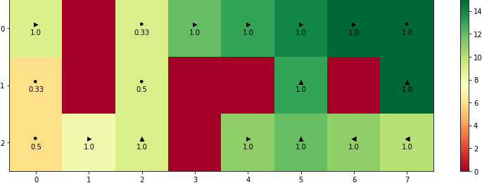
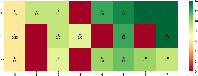
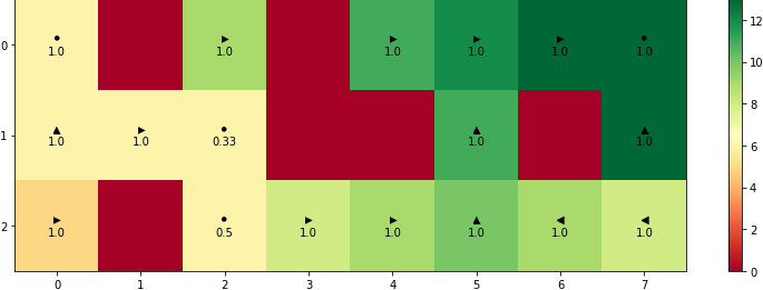
There are two interesting conclusions that can be drawn from the figures above:
- The places where the highest probability among all possible actions is $0.5$ or $0.33$ correspond to the case of having $2$ or $3$ equally good choices. For example, if you stay at $(0, 2)$ in the top figure you can either wait for $2$ turns or to move one bin to the left/down and come back. We have to mention that due to the fact of working with finite precision numbers it is always possible that some actions get higher probability than other actions even if they are equally good.
- The high penalty for passing through \(s=(1,7)\) forces a person at position \(s=(2,7)\) to pick a longer c-shaped trajectory around the monster and the static obstacle.
Summary
The presented map navigation problem was solved by assuming that the decision to which state to move depends only on the current state which allowed us to derive a sequence of simple optimization subproblems for every time step. These problems were a specific case of the Bellman equation and were solved by using a L-BFGS-B algorithm/gradient ascent method. The proposed solution does not allow a person to learn a strategy how to navigate through another unknown map or to handle unexpected events. Fortunately, there are other approaches to tackle this problem which could be discussed in detail in another article.