Table of Contents

1. Introduction
2. Model Architecture
   • 2.1 Calculating Raw Scores
   • 2.2 Mapping Raw Scores to Distribution Parameters
3. Model training
   • 3.1 Loss function
   • 3.2 Estimating Initial Scores
   • 3.3 Growing Trees: The Objective Function
   • 3.4 Taylor Approximation of the loss function
4. Model evaluation
   • 4.1 Calibration plot
   • 4.2 Probability integral transform histogram
   • 4.3 Relative standard deviation histogram
   • 4.4 Continuous ranked probability score (CRPS)
5. Practical Aspects of Model Training with Dask
   • 5.1 Why Dask for Distributed LightGBM Training?
   • 5.2 Cloud Infrastructure Setup on Google Cloud Platform
   • 5.3 Dask Deployment on Kubernetes
6. References

1. Introduction

In many real-world scenarios, we need more than just a single predicted value - we also need to quantify the uncertainty around it. For instance, when predicting a 30-minute trip, we might want to know: "What's the probability that this trip will last between 25 and 35 minutes?" Is it 50%? 80%? 95%? This information is crucial for decision-making.

One powerful way to capture this uncertainty for regression problems is to predict an entire probability distribution $\rho$ rather than a single point. The distribution tells us where we expect the forecasted variable to lie, and how certain we are about this expectation. A narrow distribution indicates high certainty; a wide distribution indicates more uncertainty. In this post, we use LightGBM to predict the parameters that fully describe such a distribution.

Problem Setup: Predicting Trip Travel Times

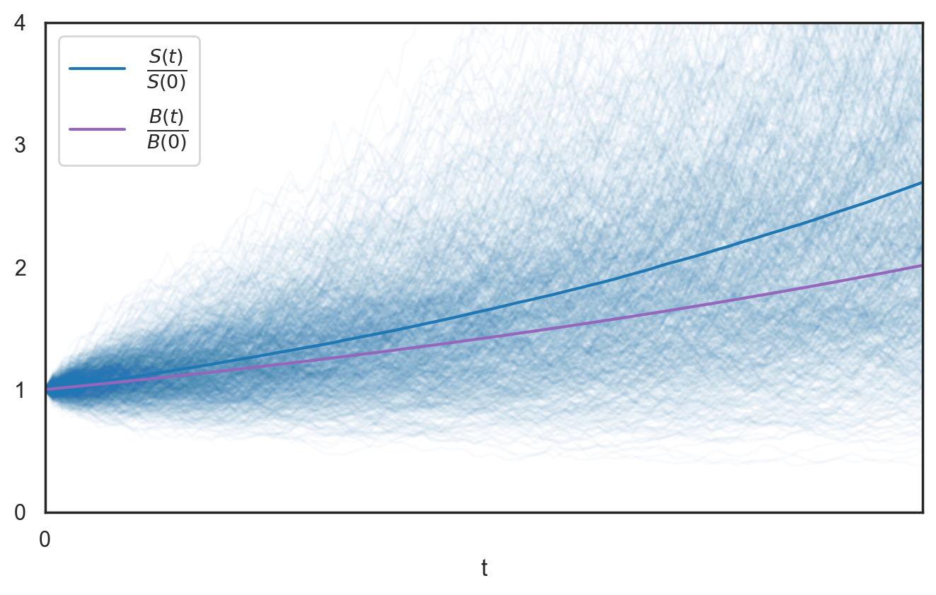
To make the discussion concrete, we focus on the problem of predicting trip travel times. Since travel times should be positive, we choose the Gamma($\alpha$, $\beta$) distribution to model the uncertainty in our predictions. Our task is to predict both distribution parameters $\alpha$ and $\beta$ (that are positive, as well) as functions of the input features $x$: e.g., distance, time of day, weather conditions, etc.

2. Model Architecture: From Inputs to Distribution Parameters

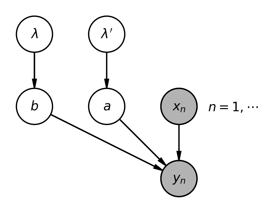
Our model transforms input features $x$ into distribution parameters $\alpha$ and $\beta$ through a two-step process. First, the gradient boosting model produces two raw scores $a_1(x)$ and $a_2(x)$ for each input $x$. These raw scores are then transformed into the positive distribution parameters $\alpha(x)$ and $\beta(x)$ using a mapping function $g$. Below, we examine each step in detail.

2.1 Calculating Raw Scores

For a single input $x$, the gradient boosting algorithm computes raw scores using the standard iterative formula:

The term on the left-hand side is the raw score for output $j$ after $T$ training iterations. The first term on the right-hand side $(a^0_j)$ is the initial score (constant baseline) for output $j$, estimated before any trees are grown. The $f^t_j$ refer to the contribution from the $t$-th tree to output $j$. In our case, $j \in \{1, 2 \}$ because we need two outputs: one will encode the mean value and the other - the rate parameter of the Gamma distribution.

Applying this formula to all $N$ points of the training dataset, gives us $2N$ outputs in total. It's convenient to organize these outputs into a $N \times 2$ matrix $A$, where each row corresponds to one data point, and the first/second column contains all $a_1$, $a_2$ values, respectively. Using matrix notation, the equation becomes:

The term on the left-hand side refers to the matrix of raw scores after $T$ iterations. The first, second column of the initial score $A^0$, is equal to $a^0_1$ and $a^0_2$, respectively. $A^t$ holds the outputs from the $t$-th pair of trees. Row $i$ $(i=1 \ldots N)$ contains the predictions for the $i$-th data point $x_i$. We'll use this matrix notation when deriving the objective function later.

2.2 Mapping Raw Scores to Distribution Parameters

The raw scores $a_1(x)$ and $a_2(x)$ can be any real numbers (positive or negative). However, the Gamma distribution parameters $\alpha$ and $\beta$ must be strictly positive. Therefore, we apply a transformation $g$ that maps real numbers to positive numbers:

The ${\rm softplus}$ function is a smooth approximation of the ReLU function that ensures positive outputs while remaining differentiable everywhere which is essential for gradient-based optimization.

The map defined in \eqref{eq:g_map} might seem like an arbitrary choice, but it has important advantages:

• Interpretable decomposition: $ {\rm softplus}(a_1) = \alpha / \beta$ represents the mean of the Gamma distribution, and $ {\rm softplus}(a_2) = \beta$ represents the rate parameter (inversely related to the scale parameter).


• Separation of roles: The first tree $f_1$ learns patterns related to the average travel time, while the second tree $f_2$ learns patterns related to variability. This separation helps the model learn more efficiently.

Alternative mappings are possible: for example, $\alpha = {\rm softplus} (a_1)$, $\beta = {\rm softplus} (a_2)$, but they don't offer the same interpretability and may lead to slower convergence during training.

3. Model training

3.1 Loss Function

To train our model, we need to define what "good predictions" mean mathematically. Instead of comparing the observed values $\{ y_i \}$ with the model point-predictions we have to compare them with predicted distributions. There are several loss-functions (aka. scoring rules) that can quantify how good is a predicted probability distribution compared to an observation. Here, we will use the negative log-likelihood of the Gamma distribution:

where $l_i$ refers to the contribution to the loss from data point $i$. The Gamma distribution evaluated at the observed trip travel time $y_i$ is denoted by $\rho (y_i | \alpha(x_i), \beta(x_i) )$. Note: In practice, you might normalize this loss by dividing by $N$, but we omit this for notational simplicity.

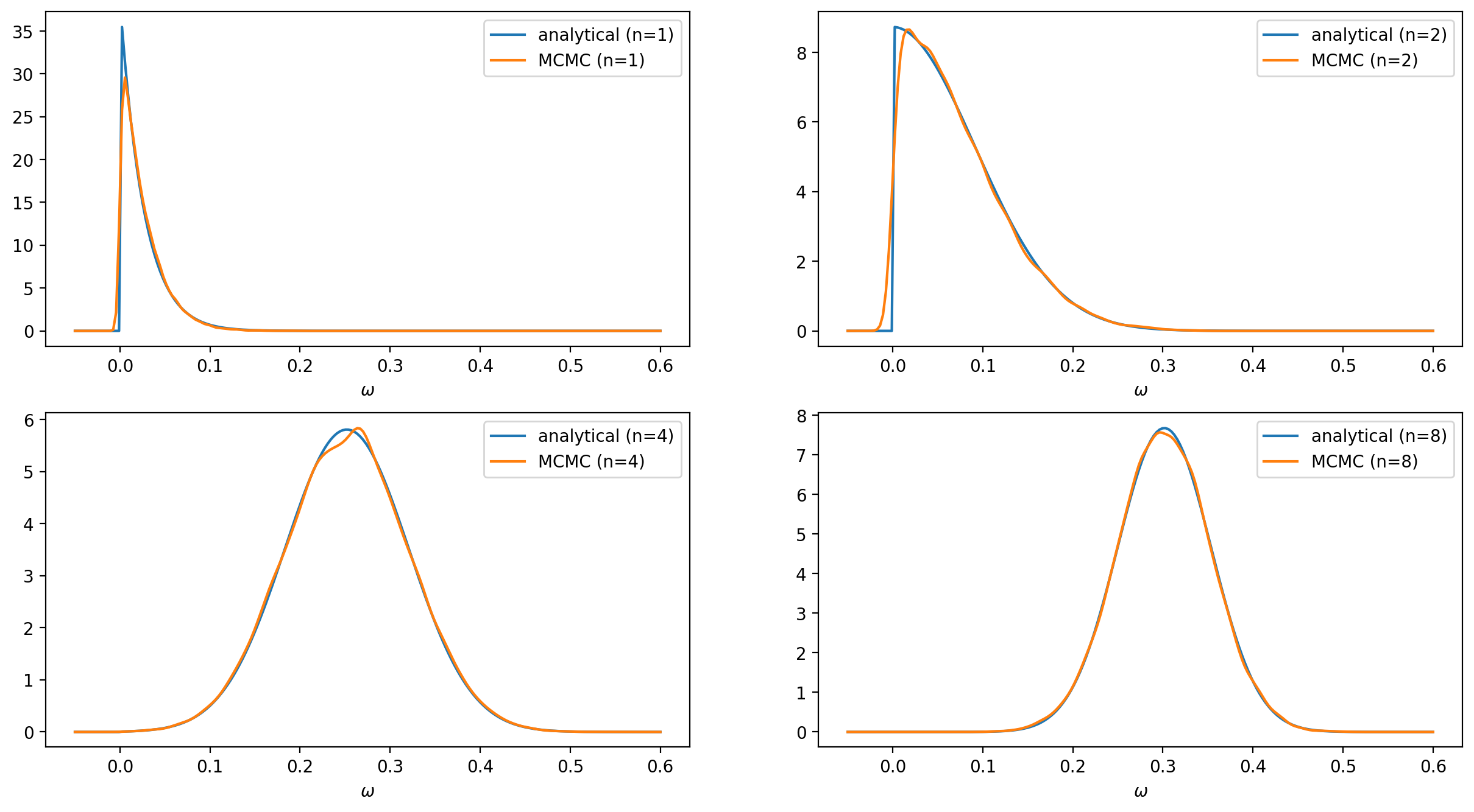
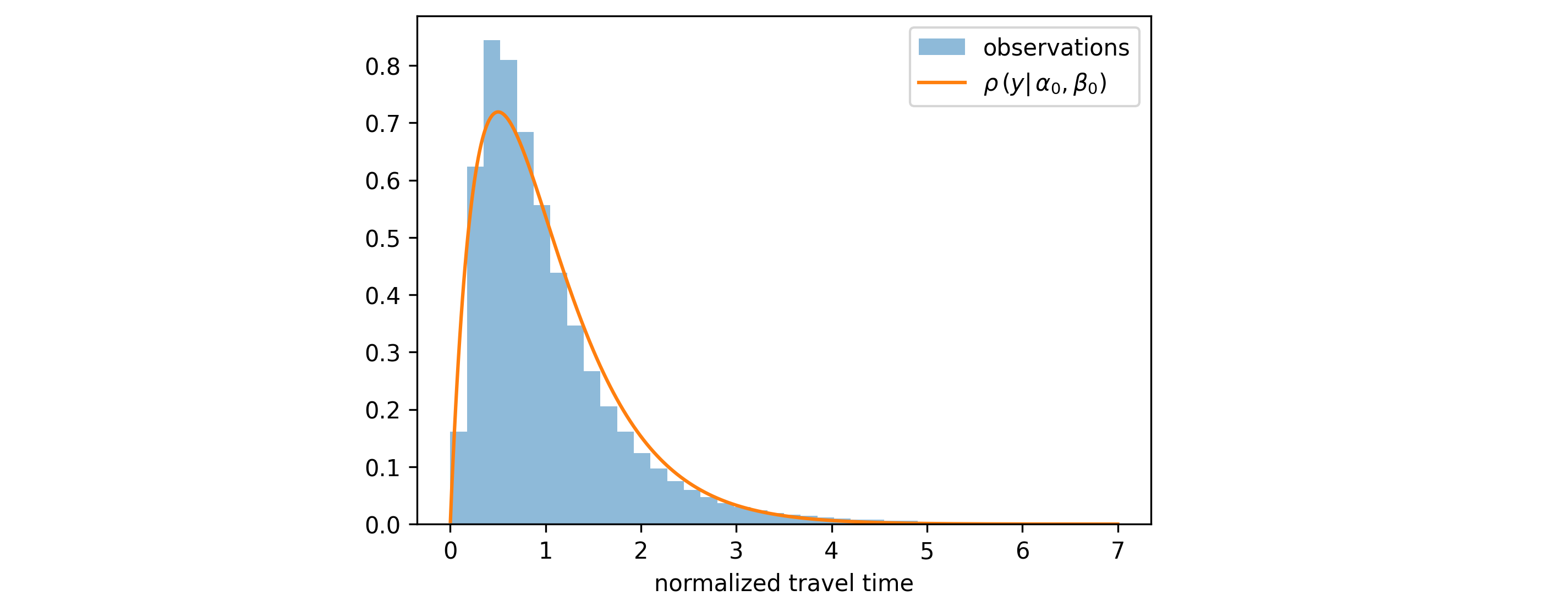
3.2 Estimating Initial Scores

Before growing any trees, we need to establish baseline predictions: the initial scores $a^0_1$ and $a^0_2$. These are feature-independent constants that provide a reasonable starting point for the iterative learning process. To find them we have to do the following steps:

• Step 1: Find the optimal constant distribution parameters $\alpha_0$ and $\beta_0$ that minimize the loss over the entire training dataset: \begin{align} (\alpha_0, \beta_0) & = \underset{\alpha, \beta }{\mathrm{arg \ min}} \sum^{N}_{i=1} - \log\left[ \rho \left(y_i | \alpha, \beta \right) \right] \end{align} This is a simple optimization problem (no features involved) that can be solved using scipy's built-in maximum likelihood estimation for the Gamma distribution.





• Step 2: Convert these optimal parameters back to raw scores using the inverse mapping $g^{-1}$: \begin{align} a^0_1 & = \rm{softplus}^{-1}(\alpha_0 / \beta_0) \nonumber \\ a^0_2 & = \rm{softplus}^{-1}(\beta_0) \end{align} where $\rm{softplus}^{-1}$ is the inverse of the softplus function.

While we use constant initial scores here, you're not restricted to this approach. You could use a simpler model (e.g., linear regression) to predict feature-dependent initial scores, as long as you use the same loss function \eqref{eq:loss_fn} and you compute initial scores for every point in the training/validation dataset before growing trees. This can give your model a head start, especially if simple linear relationships exist in your data.

3.3 Growing Trees: The Objective Function

Now comes the core of gradient boosting: iteratively growing trees to minimize the loss. To grow each tree, LightGBM requires an objective function that computes the gradient of the loss with respect to the raw scores (first-order derivatives), and the diagonal of the Hessian matrix (second-order derivatives). An explanation how the gradients and the Hessian impact the tree growth is provided in the XGBoost tutorial where an example of growing a single tree per iteration was considered, and Taylor expansion of the loss function up to the second order was applied. We would like to take a closer look at the latter step and see how it changes for our problem.

3.4 Taylor Approximation of the loss function

The foundation of gradient boosting is a second-order Taylor expansion of the loss function w.r.t. the raw scores. We recall again the matrix notation for the raw scores used in \eqref{eq:lgbm_def_matrix}. When we grow the $T$-th pair of trees we update the raw scores by adding to them the matrix $A^t$ $(t=T)$ on the right-hand side. If we assume that the values of the new matrix $A^t$ $(t=T)$ are very small then the update of the total loss $L$ should be small, as well, which justifies the application of the second-order Taylor expansion w.r.t. $A^t$ $(t=T)$: \begin{align} \label{eq:loss_taylor} L^{[T]} &= \sum^{N}_{i=1} l^{[T]}_i \\ & \approx \sum^{N}_{i=1} \Bigg( l^{[T-1]}_{i} + \sum^{2}_{j=1} \frac{dl_i}{dA_{ij}} \vast^{}_{A_i=A^{[T-1]}_i} \hspace{-13.0mm} A^{T}_{ij} \hspace{5.0mm} + \frac{1}{2} \sum^{2}_{jj'=1} \frac{d^2l_i}{dA_{ij} dA_{ij'}} \vast^{}_{A_i = A^{[T-1]}_i} \hspace{-13.0mm} A^{T}_{ij} A^{T}_{ij'} \hspace{3.0mm} \Bigg) \nonumber \end{align} There are few key observations:

• Per-sample structure: Each data point $i$ contributes independently to the loss, which is why the subscript on $l$ matches the first subscript on $A$ which refers to the $i$-th row.


• Mixed second derivatives: The last term in the second line of \eqref{eq:loss_taylor} contains mixed derivatives, i.e. terms where $ij \neq ij'$. However, LightGBM only accepts diagonal Hessian terms.

In this example you can see one of the drawbacks of growing more than one tree per iteration: we get mixed second order derivatives. Since we are asked to provide only the diagonal of the Hessian matrix in our objective function this means that we are practically dropping the mixed derivative terms from the Taylor expansion. The model loses important information that can impact the generation process of a new tree. If we were growing only one tree per iteration we would have never observed mixed second order derivatives, and this problem would not have been present. This approximation explains why we prefer some maps $g$ from raw scores $(a_1, a_2)$ to distribution parameters $(\alpha, \beta)$, like the one in \eqref{eq:g_map} to others.

4. Model Evaluation

Since we are predicting probability distributions, we would like to know if the model is able to correctly quantify its uncertainty about a prediction. For example, if the observed value lies between the predicted 10-th and 90-th percentile 80% of the times. In addition, we would like to know if the distributions are still sharp enough. To assess both properties we use different plots and metrics.

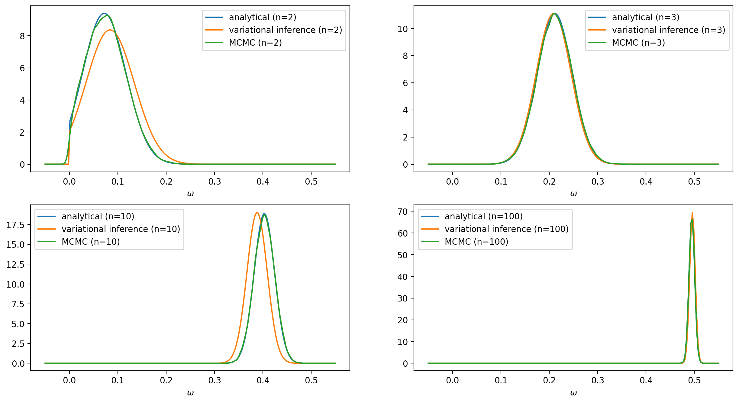
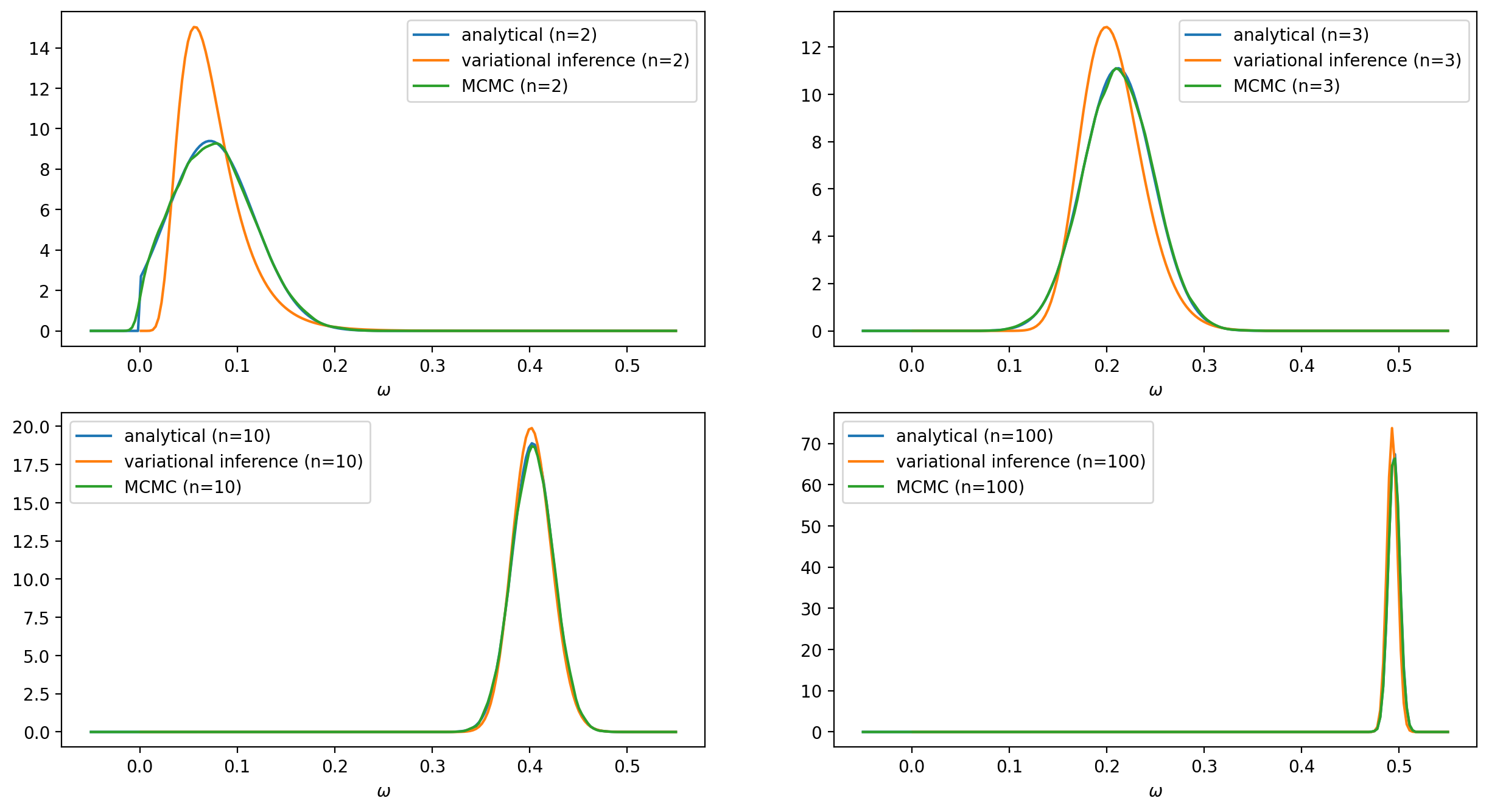
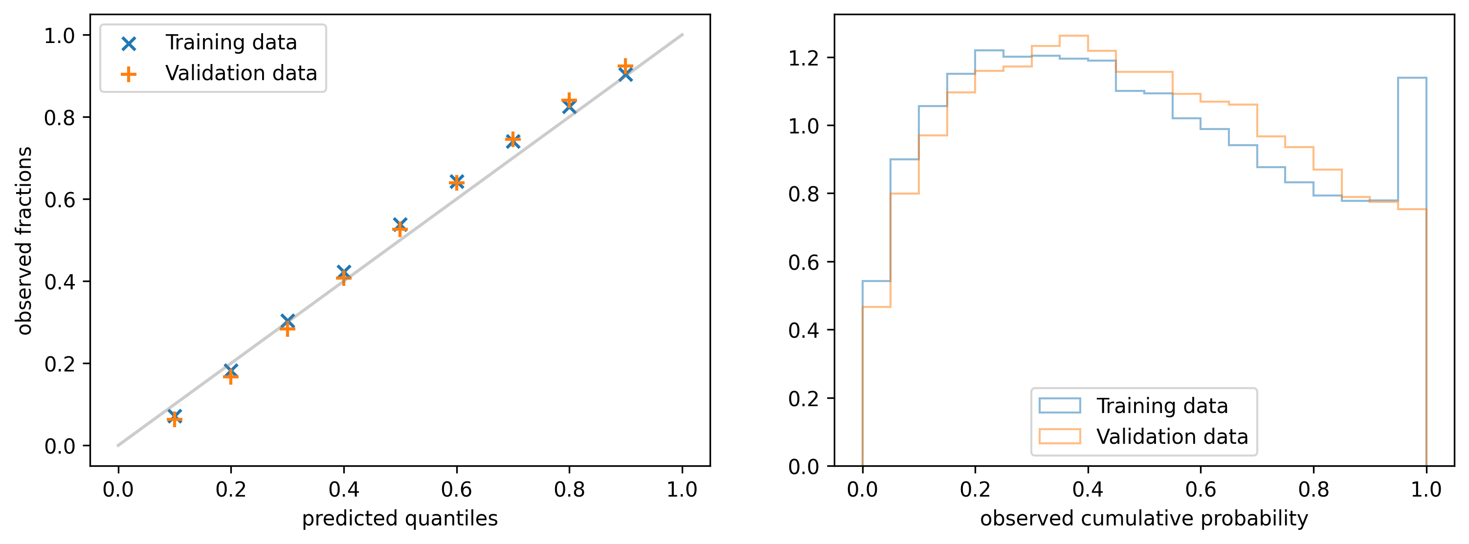
4.1 Calibration plot

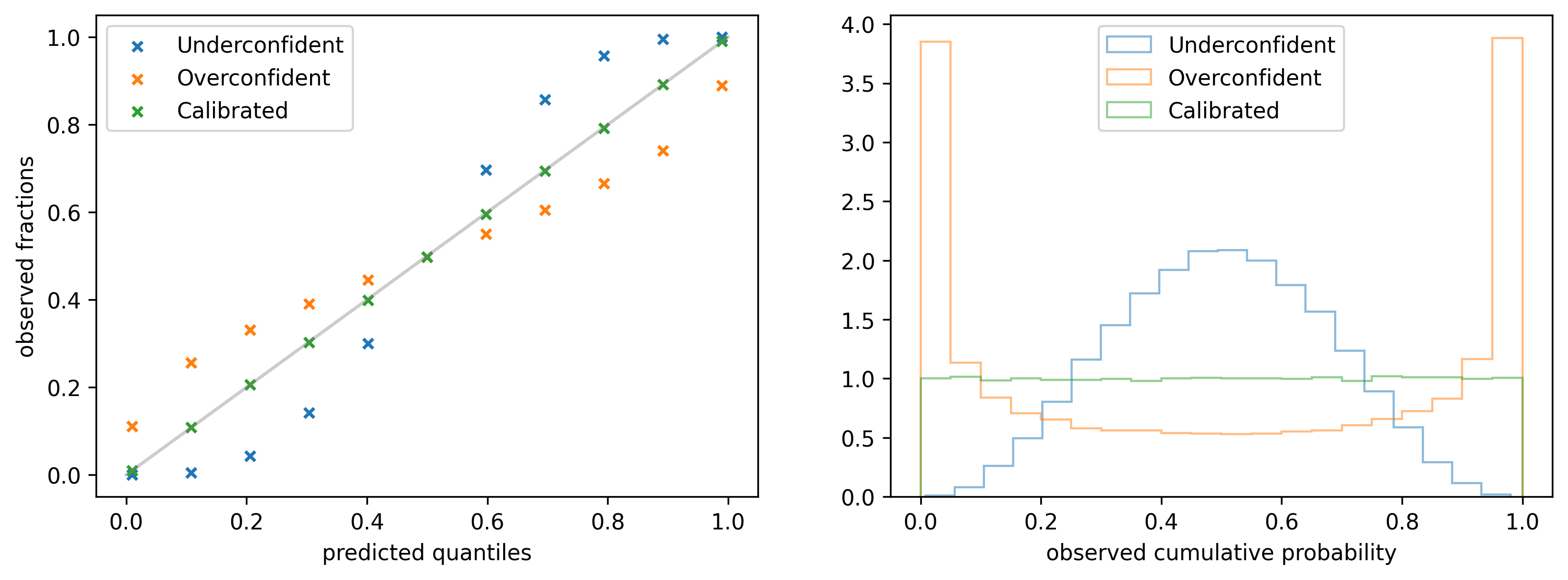
It is obtained by picking a fixed quantile $y_p$ from the predicted distribution for each data point $x$ and calculating the fraction of observations that are below $y_p$ (y-axis). The operation is repeated for a list of quantiles, e.g. $0.1, 0.2, 0.3, \ldots$ (x-axis). If the model is perfectly calibrated the observed fractions should always match the quantiles, as it is shown in the left figure below (green marks).

4.2 Probability integral transform histogram

An alternative representation of the same information is provided by the Probability integral transform (PIT): it is obtained by collecting the quantiles $q_i$ of the predicted distribution $\rho(y| \alpha(x_i), \beta(x_i))$ at which the observed values $y_i$ fall, and building a histogram. The quantiles are obtained with the following equation: \begin{align*} q_i & = \int^{y_i}_{0} \rho(y | \alpha (x_i), \beta(x_i)) dy \equiv CDF(y_i; \rho) \end{align*} where $CDF(y; ρ)$ refers to the cumulative distribution function of $\rho$ evaluated at $y$. On the right side of the figure above you can see the PIT histogram for three different types of models. For a calibrated model (green) the histogram should be uniform in the range $(0, 1)$.

If a model is too uncertain about its predictions then the histogram might have a peak at $1/2$: in the example provided above (blue) 40% of the observations lie within the predicted 0.4 - 0.6 quantile range instead of 20%. To get this number one can either calculate the area btw 0.4 and 0.6 in the histogram or look at the calibration plot and subtract the observed fractions for the same two quantiles. It follows that the predicted quantiles 0.4 and 0.6 are actually 0.3 and 0.7, respectively.

On the other hand, if a model is too certain about its predictions it is likely to observe peaks in the distribution at 0 and 1. In the third example (orange) only 50% of the observations lie in the predicted 0.1 - 0.9 quantile range instead of 80%.

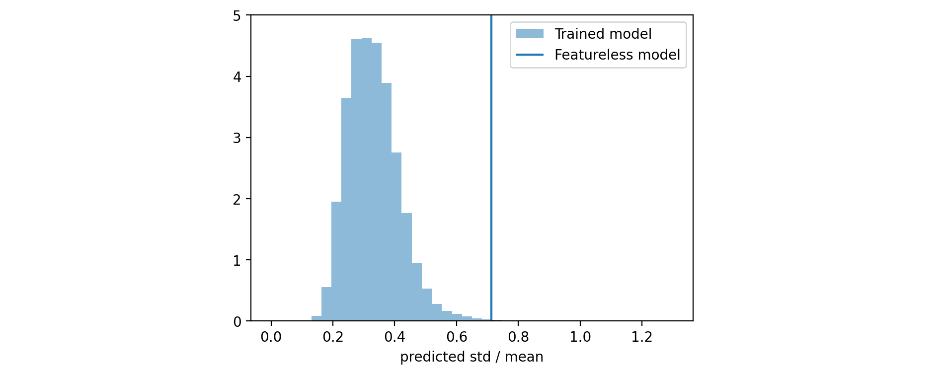
4.3 Relative standard deviation histogram

If you look at the calibration plot of the model that uses only the initial score (generated before starting to train any tree) you will see that it is already calibrated. On the other hand, we expect that this model cannot be very sharp, i.e. it predicts wide distributions with high standard deviation. Our expectation is that the sharpness should improve after each training iteration. To measure it, we can calculate the (relative) standard deviation \begin{align*} \text{rel std} & = \frac{ STD [ \rho ] }{ \mathbb{E} [ \rho ] } = \frac{1}{\sqrt{\alpha(x)} } \end{align*} or the width of a fixed interquartile range of the predicted distribution $\rho(y|\alpha(x_i), \beta(x_i))$ for each $x_i$ and build a histogram from the obtained values.

4.4 Continuous ranked probability score (CRPS)

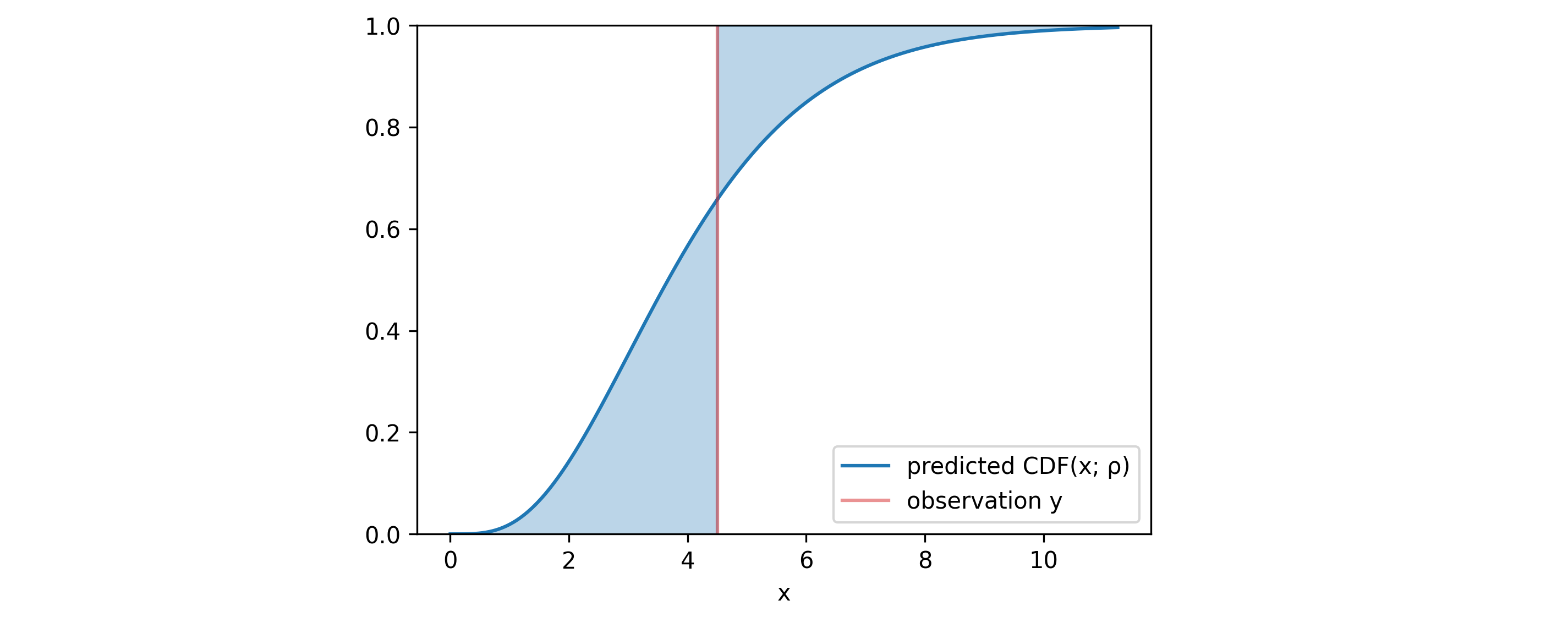
In addition to these plots, one can use a metric that simultaneously evaluates both calibration and sharpness - the CRPS. Given the observation $y$ and the predicted distribution $\rho$, it is defined as: \begin{align} CRPS(\rho, y) & = \int _{\mathbb{R}} \Big( CDF (x; \rho) - H(x-y) \Big)^2 dx \end{align} where $H$ is the Heavyside step function and $CDF(x; \rho)$ is the cumulative distribution function of $\rho$ evaluated at $x$. The blue area in the figure above represents the difference between these two functions. The area, and with it the $CRPS$ would have been minimized if the median of $\rho$ matched with the observation $y$ and if the standard deviation of $\rho$ went to $0$. This limit refers to the case of the model delivering exact point-predictions.

5. Practical Aspects of Model Training with Dask

To demonstrate our probabilistic forecasting approach, we train the model on the NYC Taxi Trip Dataset, a public dataset containing trip records with pick-up and drop-off times, locations, distances, fares, and additional metadata. While data fetching, preprocessing, and feature engineering are straightforward and well-documented in our GitHub repository, this section focuses on why we should use Dask for distributed training and what infrastructure is required to deploy the training pipeline on Google Cloud.

5.1 Why Dask for Distributed LightGBM Training?

The NYC taxi dataset's size necessitates distributed training - training on a single machine is either impossible or prohibitively slow. For distributed gradient boosting, practitioners typically choose between two main ecosystems:

• Apache Spark + SynapseML. It is a mature distributed computing framework with wide adoption but it has the critical limitation of not supporting training a LightGBM model with a custom loss-function, at least not through the PySpark API. An additional challenge is that PySpark generally discourages user-defined functions (UDFs) due to performance overhead from Python-JVM communication. Scala users might be able to overcome these limitations but this is outside of our scope.


• Dask + LightGBM. Dask is an open-source library for parallel computing that is smaller and lighter weight than Spark. It is written in Python and offers a seamless integration with other python libraries like NumPy, pandas, and Scikit-learn. The native LightGBM library supports distributed learning via Dask and since version 4.0.0 it supports custom loss functions, as well.

5.2 Cloud Infrastructure Setup on Google Cloud Platform

We will use Google cloud to create the infrastructure required to train the model:

• A service account to which we will assign different access rights.


• Google cloud storage (GCS) where we will store the training data and the artifacts of the trained model.


• A Kubernetes cluster for the training.

5.3 Dask Deployment on Kubernetes

Once the resources are ready, we can use one of the official Helm charts to set up Dask. The deployment that we will use creates a single Dask scheduler that coordinates the task execution, several Dask workers that execute the computation, and a Jupyter Lab interactive environment for development and experimentation. You can use a jupyter notebook inside Jupiter Lab to execute the data collection, data preprocessing and model training steps. In the end, you have to destroy the Kubernetes cluster since it incurs high costs.

This setup is thought more for experimentation. An automation of the training workflow can be achieved with Vertex AI where the computational resources will be automatically released (destroyed) once the training is done.

6. References

• Source code
• Introduction to Boosted Trees
• How to fix Mean Absolute Error
• Demystifying the Probability Integral Transform

In this article, we'll explore how this system works by breaking down each component in simple terms. By the end of this guide, you'll understand how to build your own intelligent conversational agent that can work with any type of document or knowledge base. The full code can be found in this Github repository.

Table of Contents

1. What is RAG and Why Does It Matter?
2. System Architecture Overview
3. Component Breakdown
4. How Everything Works Together
5. Getting Started
6. Advantages of This Architecture
7. Summary
8. Resources

1. What is RAG and Why Does It Matter?

Retrieval-Augmented Generation (RAG) is a technique that enhances AI chatbots by giving them access to specific information beyond their training data. Traditional AI models are limited to the information they learned during their training process, which means they can't access real-time information or answer questions about documents they've never seen before.

A RAG system works by first searching through your documents to find relevant information, then retrieving the most relevant pieces of text, and finally generating responses using both the retrieved information and the AI's existing knowledge. This approach solves the critical problem of knowledge cutoffs and enables AI systems to work with domain-specific information that wasn't part of their original training data.

The power of RAG lies in its ability to make AI systems more accurate, up-to-date, and relevant to specific use cases. Instead of hallucinating or providing outdated information, the AI can reference actual documents and provide citations for its responses.

2. System Architecture Overview

Our RAG system consists of several key components working together in a coordinated workflow. When a user submits a question through the Streamlit web application, the request flows through a LangGraph RAG chain that intelligently decides whether to search the vector database for relevant information. The system then combines any retrieved information with the conversation context stored in PostgreSQL before sending everything to the OpenAI GPT model for final response generation.

This architecture ensures that every response is both contextually aware of the ongoing conversation and informed by the most relevant information from your document collection. The entire system runs on Kubernetes, providing scalability, reliability, and easy management of all components.

3. Component Breakdown

3.1 LangChain & LangGraph - The AI Orchestration

LangChain serves as the foundation for building applications with large language models, while LangGraph extends these capabilities to create stateful, multi-step AI workflows. Together, they form the brain of our RAG system, orchestrating the complex dance between user input, information retrieval, and response generation.

The core logic of the graph is described in the figure above. The system works by receiving user questions and making intelligent decisions about how to respond.

• For simple queries that don't require additional context, the system might respond directly using the AI's existing knowledge (right path).


• However, for questions that would benefit from specific information, LangGraph may decide to use the tools (left path) that you have provided to gather extra information: for example, that could be a tool that executes online searches or a tool that retrieves relevant documents from an internal database. Once relevant information is retrieved, LangGraph coordinates the combination of this context with the user's original question and the ongoing conversation history, and decides whether to use another tool or to prepare a response. This orchestration ensures that responses are not only accurate based on the retrieved information but also coherent within the context of the entire conversation thread.

3.2 OpenAI GPT - The Language Model

The OpenAI GPT model serves as the core intelligence of our system, providing natural language understanding and generation capabilities that make conversations feel human-like and intuitive. The language model performs multiple critical functions within our system.

• First, it analyzes incoming user questions to determine whether additional information retrieval is necessary or if the question can be answered directly from the model's existing knowledge. This decision-making capability prevents unnecessary tool usage and improves response times for simple queries.


• In addition, when the system retrieves relevant information after using one of the tools, the GPT model synthesizes this information with the conversation context to generate comprehensive, coherent responses.

3.3 Milvus - The Vector Database

Milvus represents a specialized database technology designed specifically for storing and searching through vector embeddings, which are numerical representations of text that capture semantic meaning. This component transforms how we search and retrieve information, moving beyond simple keyword matching to true semantic understanding.

The process begins when documents are processed and split into manageable chunks, typically a few hundred words each. Each chunk is then converted into a high-dimensional vector using OpenAI's embedding model, which captures the semantic meaning of the text in mathematical form. These embeddings are stored in Milvus along with the original text and relevant metadata.

When a user asks a question, the system converts their query into the same type of vector embedding and searches through the database to find the most semantically similar content. This approach enables the system to find relevant information even when the exact words don't match. For example, a search for "car problems" might successfully return documents about "automotive issues" or "vehicle maintenance" because the vector representations capture the underlying semantic relationships.

The sophistication of vector-based search cannot be overstated. Traditional keyword searches often miss relevant information due to variations in terminology, but vector search understands context and meaning, dramatically improving the quality of information retrieval.

3.4 PostgreSQL - The Memory System

PostgreSQL serves as the memory backbone of our conversational AI system, storing conversation history and checkpoints that enable the AI to maintain context across multiple interactions. This database management system ensures that each conversation thread maintains continuity and coherence, regardless of how long the interaction continues.

The importance of persistent memory in conversational AI cannot be understated. Without proper memory management, each interaction would be isolated, forcing users to repeatedly provide context and preventing the development of more sophisticated, multi-turn conversations that feel natural and productive.

3.5 Streamlit - The User Interface

Streamlit serves as the user-facing component of our system, providing a clean and intuitive web interface for interacting with the AI assistant. This Python framework allows developers to create sophisticated web applications without extensive web development knowledge, making it an ideal choice for data science and AI applications. The biggest advantage of streamlit is the easy management of different user sessions: you can open two tabs of the same application, start two different conversations, and there will be no information leak between them.

3.6 Kubernetes - The Deployment Platform

Kubernetes orchestrates the deployment and management of all system components, providing a robust platform that handles scaling, reliability, and inter-service communication. This container orchestration platform ensures that our RAG system can operate reliably in production environments while maintaining the flexibility to scale based on demand.

Each component of our system runs in its own containerized environment, managed by Kubernetes. This approach provides isolation between services, making the system more resilient to failures and easier to maintain. If one component experiences issues, the others continue operating normally, and Kubernetes can automatically restart failed services to maintain system availability.

The platform also manages networking between components, ensuring secure communication channels and proper service discovery. When the Streamlit application needs to communicate with the vector database or the PostgreSQL instance, Kubernetes handles the routing and load balancing automatically. This infrastructure management allows developers to focus on application logic rather than deployment complexities.

For organizations planning to scale their RAG systems, Kubernetes provides horizontal scaling capabilities that can automatically add more resources during peak usage periods and scale down during quieter times. This elasticity ensures optimal performance while controlling infrastructure costs.

4. How Everything Works Together

Understanding the complete workflow helps illustrate how these components create a cohesive, intelligent system. When a user submits a question through the Streamlit interface, the application immediately saves this interaction to the conversation history and forwards the query to the LangGraph workflow engine.

LangGraph analyzes the incoming question using the OpenAI language model to determine the appropriate response strategy. For questions that clearly require specific information not available in the model's training data, the system triggers its retrieval mechanism. This involves converting the user's question into a vector embedding and searching the Milvus database for semantically similar content.

The vector database returns the most relevant document chunks, which LangGraph then combines with the original user question and the complete conversation history stored in PostgreSQL. This comprehensive context package is sent to the OpenAI GPT model, which synthesizes all available information into a coherent, conversational response that directly addresses the user's query.

Throughout this process, every interaction is preserved in PostgreSQL, ensuring that subsequent questions can build upon previous exchanges and maintain conversational continuity. The final response appears in the Streamlit interface, completing the cycle and preparing the system for the next user interaction.

5. Getting Started

The repository provides comprehensive setup instructions that guide users through both local development and production deployment scenarios. For developers wanting to experiment and modify the system, local setup allows running all components on a single machine, making it easy to test changes and understand how the components interact.

Production deployment leverages Kubernetes to provide a scalable, reliable system suitable for real-world usage. The setup process includes detailed instructions for configuring each component, managing secrets and environment variables, and establishing proper networking between services.

Essential prerequisites include obtaining an OpenAI API key for accessing the language model and embedding services, setting up a Kubernetes cluster for deployment, and basic familiarity with Docker containers and command-line tools. The system requires several environment variables including OPENAI_API_KEY for the language model, POSTGRES_CONN_STRING for database connectivity, and MINIO_URI with MINIO_ACCESS_TOKEN for vector database access.

6. Advantages of This Architecture

The modular design of this system provides significant advantages for both development and maintenance. Each component can be updated, scaled, or replaced independently without affecting the entire system, making it easier to incorporate new technologies or adapt to changing requirements.

Kubernetes provides inherent scalability that automatically adjusts to usage patterns, ensuring optimal performance during peak periods while controlling costs during lighter usage. The system can handle multiple simultaneous users without degradation, making it suitable for organizational deployment.

Cost-effectiveness comes from using efficient models and intelligent retrieval that only accesses relevant information. Rather than processing entire document collections for every query, the system precisely identifies and retrieves only the most relevant content, minimizing computational overhead and API costs.

The clear separation of concerns makes debugging and troubleshooting straightforward. Issues can typically be isolated to specific components, and the comprehensive logging throughout the system provides visibility into the processing pipeline for optimization and problem resolution.

7. Summary

This project demonstrates a production-ready approach to building conversational AI systems that seamlessly integrate with existing organizational knowledge. By combining modern AI frameworks, specialized databases, and cloud-native deployment practices, the architecture provides a robust foundation for intelligent applications that can adapt to virtually any domain or use case.

The flexibility of this approach means that organizations can customize the system for their specific needs by simply changing the data sources and adjusting the configuration. Whether building customer support tools, educational platforms, research assistants, or internal knowledge management systems, this foundation provides the scalability, intelligence, and reliability necessary for real-world deployment.

The future of AI applications is increasingly conversational, contextual, and connected to real-world information. This project provides not just a working implementation but a blueprint for understanding how these technologies can be combined effectively. By exploring the code, experimenting with different data sources, and adapting the system to specific requirements, developers and organizations can build AI applications that truly serve their users' needs while leveraging the full potential of modern artificial intelligence technologies.

8. Resources

• [1] Source code

1. Problem description

Assume that initially all investments are allocated in an asset class $B$ which has a fixed return rate $r$. A second asset class $S$ has higher average return rate $\mu$ than $B$ but comes with higher volatility: there is a chance that its returns are much lower than $r$. The goal is to transition all assets to $S$ within one year. This is done at equidistant points in time $\{t_j |j=0, \ldots N\}$ by transferring fractions $\{ \alpha_j | j=0, \ldots N\} $ of the initial investment in $B$ to $S$. For example, if we decide to do this operation once every 4 months then the fractions are described by a 4-dimensional vector $\alpha=[\alpha_0, \alpha_1, \alpha_2, \alpha_3]$ whose elements are non-negative and sum up to $1$: we sell $B$ and buy $S$ at the 0th, 4th, 8th and 12th month of the time interval. A graphical description for the case where the time span between two sell events $\Delta T$ is 4 months is provided below.

We are interested in the overall portfolio's growth $G$ in the end of the one-year interval. It is given by:

Each term in \eqref{eq:g_definition} describes the relative value growth of investments initially allocated in $B$ and then moved to $S$ at $n\Delta T$. The first fraction is the relative growth of $B$ from $t=0$ to $t=n\Delta T$ (the time we sell this asset) and the second fraction - the relative growth of $S$ from $n\Delta T$ to $N\Delta T$ (the end of the one-year window). In the previous example $\Delta T=4$ months and $N=3$.

Since the time evolution of $S$ is described by a stochastic process, the fractions $S(N\Delta T)/S(n \Delta T)$ are random variables, and hence the portfolio's growth $G$ is a random variable, as well. We want to understand how the mean, standard deviation (std) and particular percentiles of the probability distribution describing $G$ change as we change the allocation strategy $\alpha$. Intuitively, we know that achieving higher average returns is at the cost of higher std, and worse worst case performance scenarios (described by the low percentiles of the $G$-distribution). Nevertheless, there are strategies that offer the same average returns as other strategies but with a lower volatility, and we would like to identify them.

2. Time evolution of the asset classes

As mentioned in the previous section, the two asset classes $B$ and $S$ have different behaviour. The risk-free asset $B$ provides a constant return rate $r$, leading to predictable exponential growth. Conversely, the risky asset $S$ is modeled using a Geometric Brownian motion, characterized by a drift parameter $\mu$ and a volatility parameter $\sigma$. The time evolution of $B$ is straightforward, represented by the equation

For the risky asset $S$, we describe its random fluctuations over time with the stochastic differential equation

where $W_t$ is a Wiener process. The solution to this equation is given by:

Drawing the time evolution of $B_t$ is straightforward. On the other hand, to visualize the evolution of $S_t$ we simulate multiple trajectories of its stochastic process, allowing us to observe the variability in outcomes, as shown in the figure below.

3. Solution of the optimization problem

To understand how the distribution of $G$ given $\alpha$ looks like, we have to sample many trajectories of the process $S_t$, and calculate $G$ for each one of them. Then we can examine the resulting histogram of results to calculate the metrics we are interested in such as mean, std, and percentiles. In the appendix we demonstrate how to sample trajectories of $S_t$ and use them to generate samples of $G$.

In the following experiments we measure the time in units of years ($N\Delta T=1$ and $\Delta T=1/N$) and set $(r, \mu, \sigma) = (0.03, 0.09, 0.14)$ which means that the relative growths $B_t/B_0$ and $S_t/S_0$ satisfy the following relations after one year:

i.e. an investment in $B$ or $S$ is expected to yield an average annual growth of $3\%$ or $9\%$, respectively. These figures are typical for returns from a bank savings account or an index fund investment.

Given this insight, what typical values can we expect for $G$? The mean and standard deviation of $G$ should always fall between the corresponding metrics of $B_t/B_0$ and $S_t/S_0$ as shown below:

Obtaining the lowest possible mean and standard deviation is achieved by delaying the reallocation of all $B$ assets until the very end of the year, represented by $\alpha = [0 \ldots 0, 1]$. Conversely, to reach the highest limits, we reallocate all $B$ assets at the start of the year, represented by $\alpha = [1, 0 \ldots 0 ]$. This can be directly seen if we use the two $\alpha$-vectors in \eqref{eq:g_definition}:

3.1 Example: 4-step uniform reallocation

We examine the strategy of selling $25\%$ of our $B$ shares every 4 months (at the 0th, 4th, 8th, and 12th months), represented by $\alpha = [1/4, 1/4, 1/4, 1/4]$. The figure below shows the distribution of the relative growth $G$ after one year.

As expected, the mean relative return $\mathbb{E}[G]=1.062$ and the standard deviation $STD[G]=0.082$ fall within the expected ranges defined in \eqref{eq:g_inequalities}, with a $5\%$ and $10\%$ chance of the growth being below $93.6\%$ and $96.1\%$, respectively.

3.2 Arbitrary 4-step reallocation strategies

The example $\alpha = [1/4, 1/4, 1/4, 1/4]$ is just one of countless reallocation strategies. We use a Dirichlet distribution to randomly generate other $\alpha$ strategies and calculate the mean, standard deviation, and percentiles of the corresponding relative growth $G$. Results from $10,000$ strategies are plotted below.

If we look at a vertical stripe of the left figure there will be many strategies with the same mean relative growth $G$ but with different std. For instance, at $\mathbb{E}[G] \approx 1.06$, some strategies have significantly lower standard deviations than the uniform strategy (marked by a red cross). We are interested in the subset that has the lowest $STD[G]$ given $\mathbb{E}[G]$. Based on the numerical results, all these optimal strategies follow the pattern:

indicating reallocations occur only at the beginning and end of the year, with no action in the 4th and 8th months.

Similarly, when examining the 10th percentile of $G$ instead of $STD[G]$, the same pattern emerges for the optimal strategies.

3.3 Arbitrary m-step reallocation strategies

We can extend the experiment to arbitrary $m$-step reallocation strategies. For instance, we analyzed 7-step and 13-step strategies, corresponding to selling $B$ and buying $S$ every two months and every month, respectively. In both scenarios, the optimal strategy takes the form:

We expect to see the same results for any other $m$-step strategy.

4. Summary

This article explores optimal strategies for reallocating assets from a risk-free asset class to a risky one with higher returns. It uses stochastic modeling, specifically Geometric Brownian motion, to analyze the time evolution of assets and compare different reallocation approaches. By simulating various strategies, it identifies the optimal allocation that balances return and volatility. The study finds that reallocating assets only at the beginning and end of the investment period minimizes risk while maximizing return potential.

Appendix

Drawing samples from G

We can reformulate the equation for relative growth $G$ from the first section as follows:

Instead of drawing samples from the process $S_t$ we use the transformed process $X_t = log(S_t/S_0)$, known as Arithmetic Brownian Motion:

To sample a trajectory of $X_t$ we use the Euler-Maruyama method with a small step size $\delta t$:

where $\xi_t$ are independent normally distributed random variables sampled at every step. Typically, we have to use a very small step $\delta t$ to move forward in time. Since the drift $(\mu-\sigma/2)$ and diffusion $(\sigma)$ terms of the SDE are constants we can work with arbitrarily large $\delta t $. To demonstrate, consider moving from $t_0$ to $t_1$ in $N'$ steps. The step $\delta t =(t_1-t_0)/N'$ can become arbitrarily small for large $N'$:

The sum in the last line $\xi_0 + \xi_1 + \ldots $ forms a normally distributed random variable with zero mean and variance $N'$, which can be reparametrized as $\sqrt{N'}· \varepsilon$, where $\varepsilon \sim \mathcal{N}(0, 1)$. If we use this expression in the last line of the previous equation we get:

This formula allows us to sample $X_t$ at the time ordered points $(t_0, t_1, t_2 \ldots) = (0, \Delta T, 2 \Delta T \ldots)$. From each sampled $X$-trajectory we can compute $G$:

The code to generate samples of the Arithmetic Brownian Motion is provided below:

1. Problem definition
2. Simplification of the likelihood function
3. Example
   • 3.1 Standard solution
   • 3.2 Solution with reparametrized likelihood
   • 3.3 Scaling of both approaches
4. References

Employing a Variational Inference approach, we perform regression on a continuous variable $Y$ and its associated uncertainty, denoted by $STD[Y]$, utilizing a set of categorical features. Given the potential magnitude of the dataset, consisting of millions of events, we simplify the likelihood function of the model to enhance numerical stability and accelerate solutions. The implementation of this solution with Tensorflow Probability is available in the dedicated Github repository and Colab notebook.

1. Problem definition

Let’s examine the task of utilizing $M$ categorical features to forecast both the mean value and standard deviation of a target variable $Y$. A straightforward approach involves employing a linear function (augmented by an exponential or softplus link function for the non-negative standard deviation) to model both target variables. Upon applying one-hot encoding to each feature and transforming them into vectors with dimensions equal to the cardinality of the respective features, we can characterize them as follows:

where $f$ models the mean, $g$ — the standard deviation, $x_u$ — the one-hot encoded feature $u$, and $a_u$, $b_u$ — the yet to be learned weights.

The priors of the individual elements $b_{uv}$ in \eqref{eq:regr_1a} (1a) are characterized by normal distributions $\rho (b_{uv} | 0, \lambda^2_{uv})$ with a mean of zero and a standard deviation of $\lambda_{uv}$. To ensure positivity, $\lambda_{uv}$ is drawn from a Gamma distribution, $\Gamma(\lambda_{uv}| \alpha, \beta)$, where $\alpha$ is the shape parameter and $\beta$ is the rate, both constants. The priors for the weights $\alpha_{uv}$ in \eqref{eq:regr_1b} are established in an identical manner. For a comprehensive overview of the introduced variables and their interdependencies, refer to the figure below.

Let’s delve into the precise mathematical definitions of each term. The section on the left side of the graph, featuring the $\lambda$ and $b$ symbols, represents the prior distribution for the weights $b_{uv}$:

The central portion refers to the priors of the $a_{uv}$ weights, and as previously noted, they are described in an identical manner as the $b_{uv}$ weights: a simple substitution of $b$ with $a$ and $\lambda$ with $\lambda'$ suffices.

Concluding the graph is the segment dedicated to the likelihood function, $P(y| x, a, b)$, modeled as the product of normal distributions $\rho(y| \mu, \sigma^2)$ for each data point $(x, y)$. Here, $\mu$ is determined by the function $f(x,b)$ in \eqref{eq:regr_1a}, and $\sigma$ is determined by $g(x,a)$ in \eqref{eq:regr_1b}.

2. Simplification of the likelihood function

With Tensorflow Probability, defining the joint-probability distribution function and its log-probability is straightforward, and the application of the variational inference approach is exemplified in the subsequent section.

Unfortunately, this implementation experiences escalating convergence times as the dataset size grows. To mitigate computational demands, a time-saving strategy involves simplifying the log-likelihood expression. Subsequently, we can substitute the original likelihood distribution in the solution with a newly devised custom distribution object housing the adjusted log-likelihood expression.

When dealing with only $M$ categorical features, the data points in the training dataset can be organized into a finite number of groups. Each group corresponds to a unique combination of values that the categorical features can take. The total number of groups, $N$, is equal to or less than the product of the cardinalities of the features. For example, if we have a categorical feature that can take $2$ unique values and another one that can take $4$ unique values, the total number of groups should be $8$. Here, the index $i$ denotes the group, and $j$ represents an index within that group. All observations can be expressed as $\{ (y^{(ij)}, x^{(ij)}) | i = 1, \ldots N, j = 1, \ldots N_i \}$, where $N_i$ denotes the number of elements in group $i$, and $x^{(ij)}$ refers to all categorical features of observation $(ij)$. Since all elements within the same group $i$ share identical categorical features, we can simplify $x^{(ij)}$ to $x^{(i)}$.

The likelihood function in \eqref{eq:likelihood} could be rewritten in the following form:

The last line of the equation was derived by adding and subtracting $\mathbb{E} [y^{(i)}]^2$ and regrouping the terms.

The derivation of the log-probability for both the likelihood component and the complete joint-probability distribution function \eqref{eq:likelihood} is straightforward. All summations involved are solely over the $N$ distinct groups. Within each group, the observed target values $y^{(ij)}$ are replaced with the group mean, $\mathbb{E}[y^{(i)}]$, and standard deviation, $STD[y^{(i)}]$. The resulting number of elements $N$ is considerably smaller than the total count of original observations $\sum_i N_i$.

3. Example

We explore a scenario of having a target variable $Y$ whose mean and standard deviation can be linearly regressed by two categorical variables $f0$, $f1$ with cardinalities of $2$ and $4$, respectively (and with a softplus link function applied to the standard deviation). The figure below provides a sample of the generated data:

3.1 Standard solution

To build the model (the joint probability distribution in \eqref{eq:likelihood}) we can use the code snippet below:

Since we are using the Variational inference approach to solve the problem, we have to construct a surrogate posterior for $\lambda_{uv}$, $\lambda'_{uv}$, $a_{uv}$, $b_{uv}$, as well. For simplicity, we assume that that there are no correlations between the variables. This reduces the posterior description to the product of univariate distributions of the normally distributed weights $a_{uv}$, $b_{uv}$ and log-normally distributed $\lambda_{uv}$, $\lambda'_{uv}$.

The code snippet below demonstrates how the model is trained with (method=aggregated) and without (method=standard) the likelihood simplification. Between the two approaches there are almost no differences, except the use of build_model_agg_data() and build_model() to construct the likelihoods, and the different input data.

3.2 Solution with modified likelihood

We can use the same definition of the priors and the surrogate posteriors from the previous solution. The only difficulty is plugging in the new likelihood function into the joint distribution. To achieve this we create a new class derived from the standard AutoCompositeTensorDistribtuion Tensorflow class. We are interested only in the log_prob() method of this class. The method to sample values from the distribution is defined only because Tensorflow uses it to infer the right dimensions of the sampled values (so it is fine if we define it to return only zeros).

The model (joint probability distribution) is build similarly to the model from the standard solution:

3.3 Scaling of both approaches

One can use this Colab-notebook to check if the predicted mean and standard deviation of the target variable for all feature combinations between both models are the same. By increasing the dataset size one can see that the computation time of the solution employing the modified likelihood is constant. On the other hand the computation time of the standard solution significantly increases.

4. References

• Source code: https://github.com/ImScientist/ilovetfp
• Colab notebook: https://colab.research.google.com/drive/11c8W9Sy3GleRkK7d6xs081Tv3tnYafhf?usp=sharing

Table of Contents

1. Creating and exposing tf models as REST APIs
2. Kubernetes deployment
   • 2.1 Tensorflow serving
   • 2.2 Prometheus
   • 2.3 Grafana
3. References

1. Creating and exposing tf models as REST APIs

To keep things simple we use trivial models, like f(x)=x/2+2 but the idea can be applied to any subclass of tf.Module that has the .save() method. A minimal example is provided below:

In the directory where the model is saved you can find a saved_model.pb file. It stores the TensorFlow model, and a set of named signatures, each identifying a function that accepts tensor inputs and produces tensor outputs. Whereas tf.Keras models automatically specify serving signatures, for custom modules you have to declare them explicitly, as described here. To get an overview of the available signatures you can use the saved_models_cli in your cli. Usually, you will only have and need the serving_default signature. For the example presented above you can obtain the inputs and outputs of the serving_default signature with the following command:

As a next step, we use the official tensorflow/serving image to expose the saved models as a REST API (you can use the same image to make grpc calls against the models but this won’t be covered here). An example, how to run the container, mount the saved model (assuming that it is stored in $(pwd)/models), and make a REST call is provided below:

In this example we made 3 predictions of f(x)=x/2+2 for x=0,1,2. Note that in the POST request we had to specify the signature name serving_default and to make the input data compliant with the signature definition.

To serve multiple models we do not only have to mount them in the image but also have to specify a config file that maps the model location to a service path. For example, if we have 3 models mounted in the /models directory, as described below,

we can use the following configuration (mounted in /models/models.config):

You can copy the content in /models from here. To start the service we will use the same tensorflow/serving image but with few extra arguments:

• The model_config_file_poll_wait_seconds flag instructs Tensorflow Serving to periodically poll for updated versions of the configuration file specified by the model_config_file flag.
  
  
• The version_labels section of the config file allows us to map different model versions to the same endpoint. In this example, calling the endpoints /half_plus_ten/labels/stable and /half_plus_ten/labels/canary is equivalent to calling /half_plus_ten/versions/1 and /half_plus_ten/versions/2, respectively.
  
  
• The allow_version_labels_for_unavailable_models flag allows us to assign a label to a version that is not yet loaded.
  
  

In this example the following service calls are possible (you can pick each one of the three MODEL_PATH by commenting out the other two):

2. Kubernetes deployment

For simplicity, we use a Kubernetes cluster deployed on a local machine. This prevents us, for example, to simulate exactly how the new tensorflow models are mounted and served but all other configurations presented below can be used for the cloud deployment.

To reproduce the steps listed below, you need a local Kubernetes installation, like Docker Desktop or Rancher Desktop, and the helm package manager that automates the deployment of software for Kubernetes.

2.1 Tensorflow serving

We create a single deployment that is exposed to the other components in the cluster through a service. In the ideal case, the exported models should be made available to the tf-server pods by mounting them as volumes. Instead, the pods in the deployment will be running containers that already contain the models. The Dockerfile that creates them is given below:

We can create the container, the kubernetes namespace, deployment and service with the following commands:

where the content of tf-serving.yaml is given below:

In this repository you can also find the corresponding helm chart. From the yaml file we can see that:

• We are pulling the locally stored tensorflow server image by setting pullPolicy: Never (line 21). This line should be changed if we are using a cluster on the cloud (in addition to pushing the tf-server:1.0.0 image to a container registry).
  
  
• We provide a monitoring configuration to the server by using the rest_api_port flag and the monitoring_config_file flag (line 24, 27). The latter flag points to the /models/monitoring.config file that has the following content:
  
  
• All metrics that can be scraped by Prometheus are accessible at path /monitoring/prometheus/metrics and port 8501. You can see them by browsing to http://localhost:8501/monitoring/prometheus/metrics.
  
  
• We are using a service of type LoadBalancer (line 42). If the service is intended to be used only by other components in the same cluster then we could change the type of the service to ClusterIP. We should be able to make API calls to the service in the same way as we did in the previous section.
  
  

2.2 Prometheus

We will use helm to install all Prometheus components. Since it provides us with a working application out of the box we do not have change its default settings. We only have to provide the instructions how to discover the pods of the Model Server and extract information from them. We can do this by:

• storing the configurations as a secret in the same namespace where Prometheus is deployed and providing the secret name and key to Prometheus.
  
  
• defining the configurations to be managed by the Helm. In this case a change of the configurations requires a new release version.
  
  

It defines a scrape job that looks for pods with the label app: tf-serving (line 13) in the tfmodels namespace (line 17) and every 5s it checks for new data by calling /monitoring/prometheus/metrics on port 8501. To install all Prometheus components execute:

You should get a message telling you under which DNS from within the cluster Prometheus can be accessed.

To access Prometheus from outside the cluster execute: kubectl -n monitoring port-forward svc/ 9090:9090 (the service name is obtained from the panel above). After few minutes when all Prometheus components are installed you can access the Prometheus UI at http://127.0.0.1:9090. You can execute the query :tensorflow:serving:request_count and check how the graph changes after making several API calls to the tf model service.

2.3 Grafana

We will use helm to install Grafana. No additional configurations are required:

You should automatically get the following instructions how to access the Grafana dashboard (note that in the panel below the kubectl namespace flag is skipped; you should not skip it):

To access Grafana from outside the cluster execute kubectl -n monitoring port-forward svc/grafana-chart 8080:3000 and browse to http://127.0.0.1:8080 to access the service. You can add Prometheus as a datasource by using the previously obtained prometheus DNS name as a datasource URL: http://.monitoring.svc.cluster.local:9090

Now you should be able to create your first dashboard by using the metric :tensorflow:serving:request_count and Prometheus as a data source.

To remove all components that you have installed execute:

3. References

• Specifying signatures of tf.models during export
• Helm installation
• Prometheus scrape configuration
• Source code

Table of Contents

1. Infrastructure
2. Deployment with Google cloud SDK
3. Deployment with terraform
4. Resources

1. Infrastructure

We will create the following resources in Google cloud:

• Bucket in cloud storage that will be used as artifact storage
• PostreSQL DB in cloud SQL that will be used as mlflow backend db
• Container registry (GCR) that will host our custom mlflow image defined here
• Service account (and json-key) with access to GCS and cloud SQL
• Service account (and json-key) with access to GCR (used by the Google node pool to pull images from GCR)

The kubernetes cluster contains:

• Kubernetes Secret that contains credentials of the service account with GCS and SQL access, as well as access to the backend db
• Kuberentes Configmap
• Kubernetes Deployment where each pod holds two containers:
• cloud sql auth proxy container that creates a secure connection to the PostgreSQL DB
• mlflow server that connects to the PostgreSQL DB via the cloud sql auth proxy. We use a custom build image that is defined here.
• Kubernetes Service

2. Deployment with Google cloud SDK

We will rely on the Google cloud SDK to create the resources of interest. To run the commands below you need to have gsutil, gcloud and OpenSSL CLIs installed.

• Setup environment variables:
• Create the required resources in Google cloud (except the kubernetes cluster): Unfortunately, I am not able to create a kubernetes cluster with the gcloud sdk so you have to use the UI to create it.
• Creation of the Kubernetes cluster components. You have to change the kubectl context: There is an option for local deployment with docker-desktop. In this case you have to create a docker-registry secret that porvides access to the container registry with our custom mlflow image: The commands for the creation of the remaining components are the same both for the local and for the Google cloud deployment:
• Test if everything works:
  To test if the Mflow server is running you can execute the following python code snippet and verify through the mlflow UI that the results are logged. In the experiment definition you will see that we are using the GCS_CREDENTIALS to store the artifacts in GCS. You also have to change the tracking URI.

3. Deployment with terraform

To understand the following code snippets you should look at the source code provided here.

• Install the terraform version manager. We will work with version 1.2.7:
• Set the project, region and zone in ./terrafrom/variables.tf and authenticate: The following command will create the required infrastructure (backend db, cloud storage, kubernetes cluster and service accounts). It will also create the namespace mlflow and add to it a config-map and a secret with all relevant credentials for the service.
• To deploy the service, we first have to build a mlflow-server image (content in ./mlflow_server directory) and push it to the container registry in our project. We will use Google cloud build. As a result the image gcr.io/${PROJECT_ID}/mlflow:${TAG_NAME} should be created.
• The remaining components that have to be created are described in kubernetes/mlflow.yaml. We have to change the image of the mlflow-server-container (line 21) to point to the image that we have created in the previous step. We can use kubectl to crete the missing components:

4. Resources

• Using Google Container Registry (GCR) with Kubernetes

1. Stochastic processes and State space models

A stochastic process can be defined as a collection of random variables $\{Z_t\}$ with a time index $t$. To obtain some information from it, we often make observations $\{ y_t \}$ at different times that are noisy and deviate from the exact values $\{ z_t \} $. This type of problem is often described through state-space models where the observations $\{ y_t \}$ are described as samples of an observation process $\{ Y_t \}$ that depend linearly on the state process $\{ Z_t \}$. A graphical representation of the idea is given in the figure below:

To make everything more understandable, we will consider the local level model with a constant drift:

which is constructed with the help of the normally distributed random variables $\varepsilon_t$, $\eta_t$, and with the constant $\omega$. Due to the noise term $\varepsilon_t$ our observations can be slightly below/above the true value of $Z_t$. We can eliminate $Z_t$ dependency in $Y_t$:

Since $Y_t$ is a linear combination of Gaussian random variables it is also Gaussian with the following properties:

where $\delta_{mn}$ is the Kronecker delta which is equal to $1$ if $m=n$ and to $0$ otherwise. One can also show that $\{ Y_t \}$ is a Gaussian stochastic process which means that the joint probability distribution of every sampled trajectory $\mathbf{y}$ $(\mathbf{y} = y_1 \ldots y_T)$ can be described as a multivariate normal distribution $\rho_{\mathcal{N}}(\mathbf{y} | \mathbf{\mu}, \Sigma)$ with mean $\mathbf{\mu}$ and covariance matrix $\Sigma$:

Because $\Sigma$ is not a diagonal matrix we cannot factorize $p(\mathbf{y})$ into a product of the distributions for each point of the trajectory $\mathbf{y}$. In fact, we can show that knowing $y'$ measured at $t' < t$ influences our measurement $y$ at $t$. We just have to compare the normal distributions $p(y|y')$ and $p(y)$:

If we compare $(4e)$ and $(4f)$ we see that the variance of $p(y|y')$ is smaller than the variance of $p(y)$, i.e. knowing $y'$ decreases our uncertainty about $y$. A comparison of both means in $(4c)$, $(4d)$ shows us that any deviation of $y'$ from its expected value $\omega t'$ shifts the expected value of $y$ in the same direction.

In real world applications we might have data from multiple trajectories of the same stochastic process. For the process that we have considered we can see that the joint probability distribution of the points from all trajectories factorizes into a product of joint probability distributions for every trajectory:

where $\mathbf{y}^m$ refers to the values of the $m$-th trajectory. In other words, the trajectories do not interfere with each other.

2. Example

We consider again the problem of finding out the growth rate $\omega$ of the trees in the Black Forest national park by using a dataset that contains two measurements of the height of every tree (and its age) taken at different points in time that differ by several years. The trees growth will be described by the local level model with constant drift $\omega$ that was defined in $(1)$ (we will also close our eyes for the fact that the tree heights may become negative. In the end we are just imagining things and our imagination should not any have boundaries). Our prior belief about the non-negative three growth rate $\omega$ is described through an exponential distribution:

where $\Theta (\omega)$ is the Heavyside step function that is equal to $1$ for $\omega > 0 $ and $0$ otherwise. The variances of $\varepsilon_t$ and $\eta_t$ will be considered as known and won’t be deduced from the data.

2.1 Analytical solution for a single tree

In this case we have only one trajectory with two points. We will denote by $y$, $y'$ the height of the tree taken at $t$, and $t'$ $(t > t')$, respectively. The corresponding trajectory $\mathbf{y}$ will be $\mathbf{y} = (y, y')$. The joint distribution of the trajectory $p(\mathbf{y})$ is given by the two-variate normal distribution $(3)$. It can be also interpreted as the likelihood function of getting the trajectory $\mathbf{y}$ given that the tree growth rate is $\omega$. We can use the Bayesian theorem to combine our prior belief about the growth rate in $(6)$ with the likelihood function $p(\mathbf{y})$:

where $C$ is a normalization constant. As in the example from the previous blog post, the posterior is a Truncated Normal distribution. To get this result we just have to use the definition of the prior $p(\omega)$ and the likelihood $p(\mathbf{y})$, invert the 2x2 covariance matrix $\Sigma$ and regroup the terms. The longer the time-series is, the bigger is the $\Sigma$ matrix that has to be inverted.

2.2 Analytical solution for multiple trees

We will denote by $y^m$, $y'{}^m$ the height of the $m$-th tree $(m = 1 \ldots M)$ taken at $t_m$, and $t'_m$ $(t_m > t'_m)$, respectively. The corresponding trajectory $\mathbf{y}^m$ will be $\mathbf{y}^m = (y^m, y'{}^m)$. By making use of $(5)$, the likelihood function of all measurements is given by:

The posterior distribution of $\omega$ obtained after taking into account the information of the height measurements of all trees is given by:

where all terms in the sums in $(9b)$, $(9c)$ are defined in $(7b)$, $(7c)$.

2.3 Numerical solution

To solve the problem numerically we will use the MCMC implementation in TensorFlow Probability. The training data is obtained through generating multiple trajectories from $(1)$ and picking two random points from each one of them: the time difference between the different pairs of chosen trajectory points can be different. The exact details of the data generation, model definition and model training are provided in this GitHub Gist.

Here we will only briefly explain the part of the code responsible for the model definition. The tfd.JointDistributionSequentialAutoBatched() concatenates the $\omega$ prior (first element in the list) with the likelihood function, as described in $(9a)$. The likelihood function is a product of $M$ two-variate normal distributions. To verify that the $M$ two-variate random variables are independent, as expected in $(5)$, we can sample many values from them, calculate the covariance matrix and confirm that it only contains $M$ 2x2 non-zero block-matrices on the diagonal. An example can be found here.

The analytical and numerical results for various numbers of trees are shown in the figure below. The impact of the prior on the $\omega$ posterior can be seen through the vertical cut at $\omega = 0$.

3 Final remarks

We have managed to solve a simple time series problem both analytically and numerically using the TensorFlow probability library. The code provided in the Gist can now be easily extended to longer time series.

4 Resources

• [1] Source code
• [2] Covariance matrix calculation of the likelihood function

• explain the measure commonly used to quantify the difference between two distributions: the Kullback-Leibler divergence
• apply the variational inference and the MCMC approach to an analytically solvable problem

Table of Contents

1. Variational inference approach
2. Example
3. Final remarks
4. Resources

1. Variational inference approach

We are interested in the posterior distribution p of the parameters $\{ \omega_m \vert m =1, \ldots M \} $ of a model that is supposed to predict the outcome $y$ from the provided features $x$ \begin{align} \label{eq:init_eq} p \big( \omega | Y, X\big) & & \omega = [ \omega_1, \ldots \omega_M ]^T \end{align} by taking into account the new information from $N$ observations $(Y, X) \equiv \{( y^{(i)}, x^{(i)} ) \vert i = 1, \ldots N \}$ of the model performance. We want to approximate the posterior with a probability distribution function $q(\omega, \theta )$ where $\theta $ corresponds to a set of parameters whose value has to be determined.

A common choice for $q$ is the joint Gaussian probability distribution where all $\omega_m$ variables are independent of each other: \begin{align} q( \omega, \theta ) & = \prod\limits^{M}_{m=1} q( \omega_m, \theta_m ), \\ q( \omega_m, \theta_m ) & = \frac{1}{\sqrt{2\pi} \sigma_m} \exp\bigg( -\frac{1}{2} \frac{ (\omega_m - \mu_m)^2 }{ \sigma^2_m } \bigg), \\ \theta & = [\theta_1, \ldots \theta_M]^T, \\ \theta_m & = ( \mu_m, \sigma_m ). \end{align} This means that we have to find the most appropriate mean $\mu_m$ and standard deviation $\sigma_m$ for every $\omega_m$ such that the difference between the true posterior $p(\omega | Y, X)$ and $q(\omega, \theta)$ is as small as possible.

In general, to quantify this difference we use the Kullback-Leibler divergence: \begin{align} \label{eq:DKL_definition} D_{KL}( q, p) & \equiv \int q( \omega, \theta ) \cdot \log \bigg( \frac{ q( \omega, \theta ) }{ p ( \omega | Y, X ) } \bigg) d\omega, \end{align} which is a measure of probability distance. To rewrite the equation in a numerically tractable form we apply the Bayesian rule on p: \begin{align} \label{eq:p_bayes} p \left( \omega | Y, X \right) & = \frac{ p \left( Y \big| \, \omega, X \right) \cdot \overbrace{p \left( \omega | \, X \right) }^{p(\omega)} }{ \underbrace{ p \left( Y \big| \, X \right) }_{1/C } } = p \left( Y \big| \, \omega, X \right) \cdot p \left( \omega \right) \cdot C \end{align} Since the term in the denominator depends neither on $\omega$ which is integrated over in \eqref{eq:DKL_definition} nor on $ \theta $ whose most optimal values we have to find, we can just denote it from now on as a constant $1/C$. This allows us to rewrite \eqref{eq:DKL_definition} in the following form: \begin{align} D_{KL}( q, p) &= \int q( \omega, \theta ) \cdot \log \bigg( \frac{ q( \omega, \theta ) }{ p ( \omega ) } \bigg) d\omega \nonumber \\ & - \sum^{N}_{j=1} \int q( \omega, \theta ) \cdot \log\bigg( p ( y^{(j)} | x^{(j)}, \omega ) \bigg) d\omega \nonumber \\ & - \underbrace{ \int q( \omega, \theta ) \cdot \log(C) \, d\omega }_{ \log(C) }. \label{eq:kl_divergence} \end{align} In the second line, we have assumed that the different observations $(y^{(i)}, x^{(i)})$ are independent of each other which allows us to represent $p(Y | X, \omega )$ as a product of likelihood functions $p(y^{(i)}| x^{(i)}, \omega )$ for every observation $(y^{(i)}, x^{(i)})$. This form of the equation is preferred since we can easily sample values from $q(\omega, \theta )$, $p(\omega)$, and from the likelihood $p(y^{(i)}| x^{(i)}, \omega)$.

The first term in\eqref{eq:kl_divergence} is the Kullback-Leibler divergence between the prior $p(\omega)$ and $q(\omega, \theta)$. This is the only term that remains on the right-hand side of the equation if we have not done any extra observations to correct our prior beliefs. The more observations we collect, the less the optimal $q(\omega, \theta)$ depends on our prior beliefs: in this case, the weight of the second term in \eqref{eq:kl_divergence} gains importance. The third term does not depend on$\omega$ or $\theta $ and we can neglect it. In this case, \eqref{eq:kl_divergence} reduces to the definition of the Evidence lower bound (ELBO). To gain a better intuition of the last equation we will consider the two most popular models: linear and logistic regression.

1.1 Linear regression

We can describe the likelihood function as follows: \begin{align} p ( y^{(i)} | x^{(i)}, \omega ) & = \frac{1}{ \sqrt{2\pi} \sigma } \exp \left( - \frac{ ( y^{(i)} - \hat{y}^{(i)} )^2 }{ 2 \sigma^2} \right)\\ \hat{y}^{(i)} & = \omega \cdot x^{(i)} \end{align} where the second line describes the model prediction. The second term in \eqref{eq:kl_divergence} then transforms to: \begin{align} - \sum^{N}_{i=1} & \int q( \omega, \theta ) \cdot \log\bigg( p ( y^{(i)} | x^{(i)}, \omega ) \bigg) d\omega \nonumber \\ & = \frac{1}{2 \sigma^2} \int q( \omega, \theta ) \sum\limits^{N}_{i=1} \Big( y^{(i)} - \omega \cdot x^{(i)} \Big)^2 d\omega + N \log(\sqrt{2 \pi } \sigma) \end{align} Up to a constant, the last expression is equal to the square-loss function that is weighted with the posterior distribution $q(\omega, \theta)$.

1.2 Logistic regression

We can describe the likelihood function as follows: \begin{align} \label{eq:log_reg_ex_a} p ( y^{(i)} | x^{(i)}, \omega ) & = \left( \hat{y}^{(i)} \right)^{ y } \cdot \left( 1 - \hat{y}^{(i)} \right)^{ 1-y }, \\ \hat{y}^{(i)}& = \frac{1}{ 1 + \exp( -\omega \cdot x^{(i)} ) } \end{align} The right-hand side of \eqref{eq:log_reg_ex_a} is equal to the first term if $y=1$ and to the second term if $y=0$. With these definitions, the second term in $\eqref{eq:kl_divergence}$ transforms to: \begin{align} - \sum^{N}_{i=1} & \int q( \omega, \theta ) \cdot \log\bigg( p ( y^{(i)} | x^{(i)}, \omega ) \bigg) d\omega \nonumber \\ & = - \int q( \omega, \theta )\sum\limits^{N}_{i=1} \bigg(y^{(i)} \log \hat{y}^{(i)} + ( 1-y^{(i)} ) \log (1 -\hat{y}^{(i)} ) \bigg) d\omega \end{align} which is the cross-entropy loss that is weighted with the posterior distribution $q(\omega, \theta)$.

2. Example

We will look at an analytically solvable problem that will allow us to compare the true posterior distribution of the model weights with those obtained by applying the variational inference approach.

Imagine that we have to find out the growth rate of the trees in the Black Forest national park by using the data of trees whose height $y$ and age $x$ was determined after cutting them down. Every data point is obtained from a different tree which allows us to assume that the measurements are uncorrelated (other approaches that are more tree-friendly could be presented in the future). The tree height is described through the equation: \begin{align} y & = \omega \cdot x + \varepsilon, \hspace{20mm} y, x, \omega \in \mathbb{R}, \varepsilon \sim \mathcal{N}(0, \sigma^2) \end{align} and our prior belief for the non-negative three growth rate $ \omega $ is given by: \begin{align} \label{eq:prior} p(\omega) & = \lambda_0 \exp\left( - \lambda_0 \, \omega \right) \Theta(\omega), \hspace{4.0mm} \lambda_0 > 0 \end{align} where $\Theta (\omega)$ is the Heavyside step function that is equal to $1$ for $\omega > 0$ and $0$ otherwise. Since $\omega \in \mathbb{R}$ we have dropped the redundant subscript of the components of the $ \omega $ vector defined in $\eqref{eq:init_eq}$. Even though $\omega$ and $x$ are positive, there is still a finite chance that the height of the tree will become negative due to $\varepsilon $ but in our training dataset we will have sufficiently old trees, and the probability of this happening is practically zero.

2.1 Analytical solution

The posterior distribution of $\omega$ obtained after performing the measurements $(Y, X) \equiv \{ (y^{(i)}, x^{(i)}) | i = 1, \ldots N \} $ is given by: \begin{align} p \left( \omega \big| Y, X \right) & = p \left( Y \big| \, X, \omega \right) \, p \left( \omega \right) \, C \nonumber \\ & = \prod\limits^{N}_{j=1} p \left( y^{(j)} | x^{(j)}, \omega \right) p(\omega) \, C \nonumber \\ & = \prod\limits^{N}_{j=1} \frac{1}{ \sqrt{2\pi} \sigma } \exp\left( -\frac{ ( y^{(j)} - \omega x^{(j)} )^2 }{2\sigma^2} \right) \, \lambda_0 \, \exp\left(-\lambda_0 \, \omega \right) \, \Theta(\omega) \, C \nonumber \\ \label{eq:eq_anal_a} & = \frac{1}{ \text{Norm}} \, \exp\left( - \frac{ (\omega - \tilde{\omega})^2 }{2 \tilde{\sigma}^2 } \right) \Theta(\omega) , \\ \label{eq:eq_anal_b} \tilde{\omega} & = \left( \sum\limits^{N}_{j=1} y^{(j)} x^{(j)} - \sigma^2 \lambda_0 \right) \Big/ D, \\ \label{eq:eq_anal_c} \tilde{\sigma}^2 & = \sigma^2 / D, \\ \label{eq:eq_anal_d} D & = \sum\limits^{N}_{j=1} \left( x^{(j)} \right)^2 \end{align} where in the first line we have used \eqref{eq:p_bayes}. The distribution in \eqref{eq:eq_anal_a} is also known as Truncated normal distribution: because of $\Theta (\omega)$, it is equal to $0$ for $\omega < 0$. The mean \eqref{eq:eq_anal_b} and variance \eqref{eq:eq_anal_c} can be derived through the completing the square technique. The exact value of the normalization factor can be found in the reference given above.

From \eqref{eq:eq_anal_a}, \eqref{eq:eq_anal_b}, \eqref{eq:eq_anal_c}, \eqref{eq:eq_anal_d} we can obtain the classical least-squares solution if we set $\lambda \rightarrow 0$ and $\sigma \rightarrow 0$. In the first case, we change our prior belief and assume that all positive growth rates are equally probable, and in the second case we reduce the uncertainty for the posterior distribution of $\omega$ to zero, i.e. we get a point estimation of $\omega$.

2.2 Numerical solution

To solve the problem numerically we will use the TensorFlow Probability variational inference module. We will experiment with two different variational posteriors: the Log-normal and the Truncated normal distributions. The latter will be a better fit since it has exactly the same form as the exact solution. The data points that will be used to train the model are generated from the following equation: \begin{align*} y^{(j)} & = \omega \, x^{(j)} + \varepsilon^{(j)}, \hspace{4.0mm} \omega = .5, \hspace{1.0mm} \varepsilon \sim \mathcal{N}(0, \sigma=4) \end{align*} To see clearly the impact of the prior on the predictions we have chosen a rather high value $\lambda = 200$ for the rate $\lambda$ in \eqref{eq:prior}. We will compare the results obtained from the analytical, the variational inference, and the MCMC approach for a different number of data points. The complete source code can be found here.

In the case of using a Log-normal distribution as a surrogate posterior, we cannot get as good results as those with the previous surrogate posterior. Nevertheless, the distribution $q$ still manages to follow the evolution of the mean and the standard deviation of the posterior $p(\omega |Y, X)$.

3. Final remarks

In the current example, we have only estimated the growth rate $\omega$, but we can extend both numerical approaches to estimate the standard deviation $\sigma$. Moreover, the case where there are multiple correlated height measurements of the same tree can be properly accounted for by the Tensorflow STS library, which could be demonstrated in a future post.

4. Resources

• [1] Source code

1. Real-Time Bidding ecosystem

A brief description of the RTB ecosystem is given in the figure above. When a user visits an ad-supported site each ad placement will trigger an auction. Bid requests will be sent via the ad exchange to the different bidding agents. Upon receiving a bid request, every bidding agent calculates a bid that is sent together with an ad to the Ad exchange. Finally, the winner’s ad will be shown to the visitor along with the regular content of the website. The whole process should be completed within a fraction of the second. A more detailed introduction to RTB could be found in [1,2].

2. Problem description

3. Solutions to the optimization problem

We will consider an analytically solvable case that can be used to check if our numerical solution is implemented correctly. Then we will briefly describe some of the problems that arise if we apply this approach to real data: the large system of equations that have to be solved and the approximation of the winning bid probability distribution by using a finite number of observations. A numerical approach that addresses these two problems can be found in this Github repository.

3.1 Single click-through probability and winning bid distribution

We will assume that the winning bid distribution for every auction n can be parametrized by an exponential distribution: \begin{align} p_{S_n}(s) & = \alpha_n e^{-\alpha_n s} \hspace{4.0mm} \alpha_n > 0. \end{align} It follows that the probability to win auction $n$ if our bid is $x_n$ is given by: \begin{align} p_{W_n | x_n} (x_n) & = \int^{x_n}_{0} p_{S_n} (s) ds \nonumber \\ & = \int^{x_n}_{0} \alpha_n e^{-\alpha_n s} ds \nonumber \\ & = 1 - e^{-\alpha_n x_n}. \end{align} To make the problem analytically solvable we have assumed that the probability distribution functions to win the auctions $1, \ldots N$ and the corresponding user click-through probabilities are all the same: \begin{align} \alpha_n & = \alpha, & n\in \{ 1, \ldots N \} \\ p_{C_n} & = p_C & n\in \{ 1, \ldots N \}. \end{align} By applying the method of the Lagrange multipliers, we obtain the optimal bid price $x_n$ and the expected amount of money spent to be: \begin{align} x_n & = \frac{1}{\alpha} \ln \Big( \frac{N \cdot p_C}{ N \cdot p_C - N_C } \Big), \hspace{4.0mm} n\in \{ 1, \ldots N \} \\ \mathbb{E}(M) & = \frac{N_C}{p_C} \frac{1}{\alpha} \ln \Big( \frac{N \cdot p_C}{ N \cdot p_C - N_C } \Big). \end{align} In real situations, we expect that $N \cdot p_c \gg N_c$ (i.e. we have to win only a small fraction of all auctions to achieve the goal of getting $N_c$ clicks) which allows us to expand $\log ()$ around $1$: \begin{align} x_n & \approx \frac{1}{\alpha} \frac{N_C}{N \cdot p_C}, \\ \mathbb{E}(M) & \approx \frac{1}{\alpha}\frac{N^2_C}{N \cdot p^2_C} . \end{align} Since $1/\alpha$ is the mean value of the exponential distribution function and $N_c/(N \cdot p_c) \ll 1$, it follows that $x$ is a very low value, i.e. we are participating at every auction with a very low bid price. We may speculate that a similar result is obtained if we use different probability distribution functions for the prices of successful bids, i.e. that we will only be interested in the left side of the distribution because that is where the optimal value is located. This also implies that we should have a very precise description of $p_{W|x}$ for a small $x$, which in practice could be a difficult task to achieve.

3.2 Multiple click-through probabilities and winning bid distributions

The general case where each auction is described by a unique probability distribution function and where the click-through probabilities can be different for each $n$ can be solved numerically using the Python scipy library. This approach quickly becomes unfeasible if $N$ is in the order of $10^3$, which is not sufficient for more realistic cases with $N > 10^6$. To make the problem manageable by the python scipy library, we will assume that the winning bid distribution of an auction can be described by one out of $I$ different possible probability distribution functions: \begin{align} \tilde{p}_{S_i}(s) \hspace{5.0mm} i \in \{1, 2, \ldots I \}. \end{align} The same idea can be applied to the click-through probability which can only take $J$ different values: \begin{align} \tilde{p}_{C_j} \hspace{5.0mm} j \in \{1, 2, \ldots J \}. \end{align} If we look closely at the solution to the optimization problem \eqref{eq:lagrange_multipliers}, we see that the optimal bid price is the same for all auctions with the same distribution of successful bids $i$ and the same click-through probability $j$. We will denote this optimal price with $\tilde{x}_{ij}$. With these considerations in mind, the functions $f$, $g$ from the Lagrange optimization problem \eqref{eq:lagrange_multipliers} can be rewritten to: \begin{align} f(\tilde{x}) & = \sum\limits^{I}_{i=1} \sum\limits^{J}_{j=1} N_{ij} \cdot \tilde{x}_{ij} \cdot \tilde{p}_{W_i|\tilde{x}_{ij}} (\tilde{x}_{ij}) , \\ g(\tilde{x}) & = \sum\limits^{I}_{i=1} \sum\limits^{J}_{j=1} N_{ij} \cdot \tilde{p}_{C_j} \cdot \tilde{p}_{W_i|\tilde{x}_{ij}} (\tilde{x}_{ij}) - N_C, \end{align} where $N_{ij}$ is equal to the number of cases where the distribution of successful bids is of type $i$ and the click-through probability is of type $j$. With this simplification, we can numerically solve problems where $I·J <10^3$.

To demonstrate the applicability of this approach, we have considered the case where $I=3$ and $J=2$: \begin{align} \tilde{p}_{C_1} & = 0.005, \nonumber \\ \tilde{p}_{C_2} & = 0.01, \nonumber \\ \tilde{p}_{S_i} (s) & = b_i s^{b_i-1} \exp \big(1 +s^{b_i} - \exp(s^{b_i}) \big) \hspace{5.0mm} b_1 =2, \hspace{1.0mm} b_2 =4, \hspace{1.0mm} b_3=6. \end{align} The optimal solution is shown in the following figure:

3.3 Obtain probability distribution functions from real data

Under realistic conditions, we have to infer the probability distribution of successful bids from the events (prices of successful bids) in our data. We can count the number of events for a grid of $x$ values and then use spline interpolation as an approximation of the distribution function. We have applied this idea to the previous example, where instead of using the analytical form of the winning bid distribution, we have sampled data points from this distribution. From the table above you can see that the differences between the two solutions are minimal. We must take into account that the number of sampled data points per distribution is in the order of $10^6$. A lower number of sampled data points inevitably leads to a lower accuracy of the spline approximation. We also have to keep in mind that the spline approximation generates a function $h(x)$ whose second derivative $d^2h(x)/dx^2$ is zero at the boundaries of the $x$ grid. This restriction can become problematic for probability distribution functions that do not go to $0$ for $x \rightarrow 0$. One such example is the exponential probability distribution function, where the second derivative at $x = 0$ is: \begin{align} \frac{d^2}{dx^2} \alpha e^{-\alpha x} \Big\vert_{x=0} & = \alpha^3 > 0. \end{align} Another problem is that with the spline approximation we cannot guarantee that the resulting function is non-negative.

Summary

In this article, we have created a simple bidding strategy by assuming that we know the winning bid probability distribution function of each auction and the click-through probability for each advertising event. From the two examples we have considered, we have seen that the optimal solution requires precise knowledge of the left side of the winning bid probability distribution function.

Resources

• [1] Real-Time Bidding Benchmarking with iPinYou Dataset
• [2] Real-time Bidding for Online Advertising: Measurement and Analysis
• [3] Source code